Tangential displacement normal normal stress continuous (TDNNS) for linear elasticity

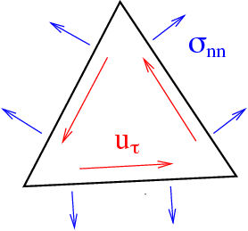
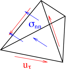
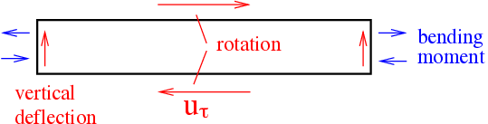
Tangential displacement normal normal stress continuous (TDNNS) for linear elasticity#

In this section we present and use the TDNNS formulation for linear elasticity. The TDNNS method fits in between the primal and dual form of the Hellinger-Reissner formulation. The degrees of freedom for the TDNNS method are:

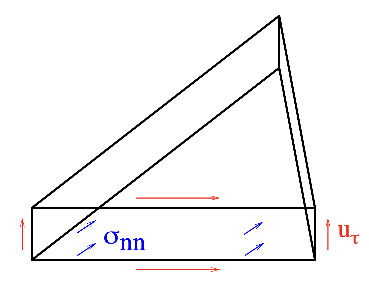
tangential component of displacement vector
normal-normal component of stress tensor

Three dofs on one edge fix rigid body modes for triangle, and six dofs on one face of a tetrahedra fix rigid body modes

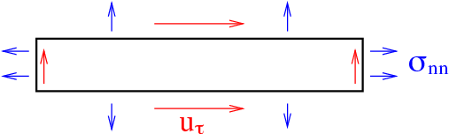
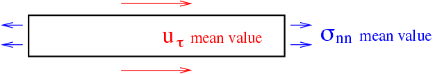
Quadrilateral/prism elements: The dofs decouple into stretching components and bending components

The divergence of \(nn\)-continuous piece-wise smooth functions#

Let \(\sigma\) be a \(nn\)-continuous finite element function, and \(f = \mathrm{div} \sigma\) be the distributional divergence, i.e.

\[\begin{align*} \langle f, \varphi\rangle & = -\int \sigma : \nabla \varphi\,dx = -\sum_T \int_T \sigma : \nabla \varphi\,dx = \sum_T \Big(\int_T \mathrm{div} \sigma\cdot\varphi\,dx - \int_{\partial T} \sigma_n \varphi\,ds\Big) \\ & = \sum_T \int_T \mathrm{div} \sigma\cdot \varphi\,dx - \sum_E \int_E [\![\sigma_n]\!] \cdot\varphi\,ds = \sum_T \int_T \mathrm{div} \sigma \varphi\,dx - \sum_E \int_E [\![\sigma_{nt}]\!] \varphi_t\,ds. \end{align*}\]

We observe that the distribution \(f\) consists of element-terms and facet-terms

\[\begin{align*} f = \begin{cases}f_T & = \mathrm{div}_T \sigma, \\ f_E & = [\![\sigma_{nt}]\!] \qquad \text{vector in tangential space}. \end{cases} \end{align*}\]

Thus, the expression

\[\begin{align*} b(\sigma, v) := \left< \mathrm{div} \sigma, v \right> = \sum_T \int_T \mathrm{div}_T \sigma v\,dx + \sum_E \int_E [\![\sigma_{nt}]\!] v_t\,ds \end{align*}\]

makes sense for functions where the tangential trace on an edge (respectively face in 3D) is well defined. This is (we cheat an \(\epsilon\) on regularity) the space \(H(\operatorname{curl})\). The canonical finite elements are the (tangential continuous) Nédélec elements (edge elements).

We take another distributional divergence of \(f = \mathrm{div} \sigma\)

\[\begin{align*} \left< \mathrm{div} f, \varphi \right> & = -\left< f, \nabla \varphi \right> = -\sum_T \int_T f_T \nabla \varphi\,dx - \sum_E \int_E f_E \nabla_t \varphi\,ds \\ & = \sum_T \Big(\int_T \mathrm{div} f_T \varphi\,dx + \int_{\partial T} f_{T,n} \varphi\,ds\Big) + \sum_E \Big(\int_E \mathrm{div}_t f_E \varphi\,ds + \int_{\partial E} f_{E,n} \varphi\Big). \end{align*}\]

Setting \(g = \mathrm{div} f\) we observe that \(g\) is a distribution of the form

\[\begin{align*} \left< g, \varphi \right> = \sum_T \int_T g_T \varphi + \sum_E \int_E g_E \varphi + \sum_V g_V \varphi(V) \end{align*}\]

with element, edge, and vertex terms

\[\begin{align*} g=\begin{cases}g_T & = \mathrm{div}_T f_T, \\ g_E & = [\![f_T \cdot n]\!] + \mathrm{div}_t f_E, \\ g_V & = \sum_{E : V \in E} f_{E,n}. \end{cases} \end{align*}\]

This functional \(g\) is well defined on the space \(H^{1+\epsilon}(\Omega)\), i.e. nearly on \(H^1(\Omega)\), which motivates the space

\[\begin{align*} H(\mathrm{div} \mathrm{div}) = \{ \sigma \in L^2(\Omega)^{d\times d}_{\text{sym}} \mid \mathrm{div} \mathrm{div} \sigma \in H^{-1}(\Omega) \}. \end{align*}\]

Normal-normal continuous symmetric matrix finite elements are (a slightly non-conforming) discretization of \(H(\mathrm{div} \mathrm{div})\).

TDNNS Variational formulation#

The primal linear elasticity problem: Find \(u\in H^1_{\Gamma_D}(\Omega,\mathbb{R}^2)\) such that for all \(v\in H^1_{\Gamma_D}(\Omega,\mathbb{R}^2)\)

\[\begin{align*} \int_{\Omega}\mathbb{C}\varepsilon(u):\varepsilon(v)\,dx = \int_{\Omega} f\cdot v\,dx + \int_{\Gamma_N}g\cdot v\,ds \end{align*}\]

can be rewritten by using the stress \(\sigma=\mathbb{C}\varepsilon(u)\) as additional unknown. Therefore the stress-strain relation is inverted

\[\begin{align*} \sigma =\mathbb{C}\varepsilon(u)= 2\mu\varepsilon(u)+\lambda\,\mathrm{tr}(\varepsilon(u))I_{d\times d},&& \varepsilon(u)=\mathbb{C}^{-1}\sigma = \frac{1}{2\mu}\mathrm{dev}(\sigma)+\frac{1}{d(d\lambda+2\mu)}\mathrm{tr}(\sigma)I_{d\times d}, \end{align*}\]

where \(d\) is is the spatial dimension of the domain \(\Omega\subset\mathbb{R}^d\), \(\mathrm{tr}(A)\) denotes the trace and \(\mathrm{dev}(A)=A-\frac{1}{d}\mathrm{tr}(A)I_{d\times d}\) the deviatoric part of the matrix \(A\). With this we obtain the formulation: Find \((\sigma,u)\) such that for all \((\tau,v)\)

\[\begin{align*} \begin{array}{cccl} &\int_{\Omega}\mathbb{C}^{-1}\sigma:\tau\,dx&-\langle \varepsilon(u),\tau\rangle &=&0,\\ &-\langle \varepsilon(v),\sigma\rangle &&=&-\int_{\Omega}f\cdot v\,dx. \end{array} \end{align*}\]

Depending on the regularity of \(\sigma\) and \(v\) the duality pairing \(\langle\cdot,\cdot\rangle\) has to be interpreted differently.

Let \(\Sigma_h\) be an \(nn\)-continuous symmetric matrix valued finite element space, and \(V_h\) a tangential continuous vector finite element space.

The TDNNS method for linear elasticity is: Find: \(\sigma_h \in \Sigma_h\) and \(u_h \in V_h\) such that \(\sigma_{h,nn}=g_n\) on \(\Gamma_N\) and

\[\begin{align*} \begin{array}{ccccll} \int_{\Omega} \mathbb{C}^{-1}\sigma_h: \tau_h & + & \sum_T \int_T \mathrm{div} \tau_h u_h + \int_{\partial T} \tau_{h,nt} u_{h,t} & = & 0 & \forall \, \tau_h\in\Sigma_h, \\ \sum_T \int_T \mathrm{div} \sigma_h v_h + \int_{\partial T} \sigma_{h,nt} v_{h,t} & & & = & \int_{\Omega} f\cdot v_h\,dx + \int_{\Gamma_N}g_t\cdot v_{h,t}\,ds & \forall \, v_h \in V_h. \end{array} \end{align*}\]

The \(b(\cdot,\cdot)\) bilinear form can be interpreted as distributional divergence:

\[\begin{align*} b(\sigma_h, v_h) = \sum_T \int_T \mathrm{div} \sigma_h v_h\,dx + \sum_E \int_{E} [\![\sigma_{h,nt}]\!] v_{h,t}\,ds = \left\langle \mathrm{div} \sigma_h, v_h \right\rangle. \end{align*}\]

References:

Error estimates#

First results were in discrete norms [Pechstein, Schöberl. Tangential-Displacement and Normal-Normal-Stress Continuous Mixed Finite Elements for Elasticity. Math. Models Methods Appl. Sci. , (2011).]

\[\begin{align*} \| \sigma - \sigma_h \|_{L_2} + \| u - u_h \|_{H^1,h} \prec \inf_{\tau_h, v_h} \| \sigma - \tau_h \|_{L_2} + \| u - v_h \|_{H^1,h} . \end{align*}\]

Recent results [Pechstein, Schöberl. An analysis of the TDNNS method using natural norms. Numerische Mathematik , (2018).] give error estimates in natural norms:

\[\begin{align*} \| \sigma - \sigma_h \|_{H(\mathrm{div} \mathrm{div}),h} + \| u - u_h \|_{H(\mathrm{curl})} \prec \inf_{\tau_h, v_h} \| \sigma - \tau_h \|_{H(\mathrm{div} \mathrm{div}),h} + \| u - v_h \|_{H(\mathrm{curl})} . \end{align*}\]

from ngsolve import *
from netgen.occ import *
from ngsolve.webgui import Draw

rect = Rectangle(10, 1).Face()
rect.edges.Min(X).name = "left"
rect.edges.Max(X).name = "right"
rect.edges.Min(Y).name = "bottom"
rect.edges.Max(Y).name = "top"
mesh = Mesh(OCCGeometry(rect, dim=2).GenerateMesh(maxh=0.5))

order = 3
V = HDivDiv(mesh, order=order, dirichlet="bottom|right|top")
Q = HCurl(mesh, order=order, dirichlet="left")
X = V * Q


(sigma, u), (tau, v) = X.TnT()

n = specialcf.normal(2)


def tang(u):
    return u - (u * n) * n


a = BilinearForm(X, symmetric=True)
a += (InnerProduct(sigma, tau) + div(sigma) * v + div(tau) * u) * dx
a += (-(sigma * n) * tang(v) - (tau * n) * tang(u)) * dx(element_boundary=True)
a.Assemble()

f = LinearForm(X)
f += -2e-4 * v[1] * dx
f.Assemble()


gf_solution = GridFunction(X)
gf_solution.vec.data = a.mat.Inverse(X.FreeDofs(), inverse="") * f.vec
gf_sigma, gf_u = gf_solution.components

Draw(gf_u, mesh, name="displacement", deformation=True)
Draw(gf_sigma[0][0], mesh, name="s11");

Hybridized TDNNS method for linear elasticity#

We can apply hybridization techniques NGSolve docu - Static condensation to retain a positive definite problem. Therefore, the continuity condition on the stress space is broken and gets reinforced weakly by means of a Lagrange multiplier. Note, that essential and natural boundary conditions again swap. The hybridized TDNNS method for linear elasticity is: Find \(\sigma_h \in \Sigma_h\), \(u_h \in V_h\), and \(\hat{u}_h\in \Lambda_h\) such that:

\[\begin{align*} \begin{array}{ccccll} \int_{\Omega} \mathbb{C}^{-1}\sigma_h: \tau_h\,dx & + & \sum_T \Big(\int_T \mathrm{div} \tau_h u_h\,dx + \int_{\partial T} \tau_{h,nt} u_{h,t} + \tau_{h,nn}\hat{u}_{h,n}\,ds\Big) & = & 0 & \forall \, \tau_h\in \Sigma_h \\ \sum_T \Big(\int_T \mathrm{div} \sigma_h v_h\,dx + \int_{\partial T} \sigma_{h,nt} v_{h,t}\,ds\Big) & & & = & -\int_{\Omega} f\cdot v_h\,dx & \forall \, v_h\in V_h\\ \sum_T\int_{\partial T} \sigma_{h,nn}\hat{v}_{h,n}\,ds & & & = & 0 & \forall \, \hat{v}_h\in\Lambda_h \end{array}, \end{align*}\]

where \(\Lambda_h\) is a finite element space living only on the skeleton (edges in 2D) in normal direction such that the normal-normal continuity is forced

\[\begin{align*} \sum_T\int_{\partial T} \sigma_{h,nn}\hat{v}_{h,n}\,ds = \sum_E\int_E[\![\sigma_{h,nn}]\!]\hat{v}_{h,n}\,ds=0. \end{align*}\]

We can write down the system matrix

\[\begin{align*} &\qquad\quad\begin{pmatrix}A & B^\top\\ B & 0\end{pmatrix}\begin{pmatrix}\underline{\sigma}\\\begin{pmatrix}\underline{u}\\\underline{\hat{u}}\end{pmatrix}\end{pmatrix}=\begin{pmatrix}0\\ \underline{f}\end{pmatrix}. \end{align*}\]

From the first equation \(\underline{\sigma}\) can be explicitly expressed in terms of \(\underline{u}\) and \(\underline{\alpha}\). This identity is inserted into the second equation leading to the Schur-complement matrix \(-BA^{-1}B^\top\). Note that \(A\) is a block diagonal matrix and thus cheap to invert

\[\begin{align*} \underline{\sigma} = -A^{-1}B^\top \begin{pmatrix}\underline{u}\\\underline{\hat{u}}\end{pmatrix},\qquad -BA^{-1}B^\top \begin{pmatrix}\underline{u}\\\underline{\hat{u}}\end{pmatrix}=\underline{f}. \end{align*}\]

from ngsolve import *
from netgen.occ import *
from ngsolve.webgui import Draw

rect = Rectangle(10, 1).Face()
rect.edges.Min(X).name = "left"
rect.edges.Max(X).name = "right"
rect.edges.Min(Y).name = "bottom"
rect.edges.Max(Y).name = "top"
mesh = Mesh(OCCGeometry(rect, dim=2).GenerateMesh(maxh=0.5))

order = 3
V = Discontinuous(HDivDiv(mesh, order=order))
Q = HCurl(mesh, order=order, dirichlet="left")
Qh = NormalFacetFESpace(mesh, order=order, dirichlet="left")
X = V * Q * Qh

(sigma, u, uh), (tau, v, vh) = X.TnT()

n = specialcf.normal(2)


def tang(u):
    return u - (u * n) * n


a = BilinearForm(X, symmetric=True, condense=True)
a += (InnerProduct(sigma, tau) + div(sigma) * v + div(tau) * u) * dx
a += (-(sigma * n) * tang(v) - (tau * n) * tang(u)) * dx(element_boundary=True)
a += ((uh * n) * tau * n * n + (vh * n) * sigma * n * n) * dx(element_boundary=True)
a.Assemble()

f = LinearForm(X)
f += -2e-4 * v[1] * dx
f.Assemble()

gf_solution = GridFunction(X)

res = f.vec.CreateVector()
res.data = f.vec - a.mat * gf_solution.vec

if a.condense:
    res.data += a.harmonic_extension_trans * res

    gf_solution.vec.data += (
        a.mat.Inverse(X.FreeDofs(coupling=True), inverse="sparsecholesky") * res
    )
    gf_solution.vec.data += a.harmonic_extension * gf_solution.vec
    gf_solution.vec.data += a.inner_solve * res
else:
    gf_solution.vec.data += a.mat.Inverse(X.FreeDofs(coupling=False), inverse="") * res

gf_sigma, gf_u, gf_uh = gf_solution.components

Draw(gf_u, mesh, name="displacement", deformation=True)
Draw(gf_sigma[0], mesh, name="s11");