8.4. Reissner-Mindlin plate

In this section we discretize and solve the Reissner-Mindlin plate (see Reissner-Mindlin and Kirchhoff-Love plates for a derivation) with two different methods and discuss the appearance of shear locking. The total energy consisting of bending and shearing reads with the vertical deflection \(w\) and the linearized rotation vector \(\beta\)

\[\begin{align*} \mathcal{W}_{\mathrm{Reissner-Mindlin}}(w,\beta) = \frac{1}{2}\int_{\Omega}\| \varepsilon(\beta) \|_{\mathbb{D}}^2 + \frac{\kappa\,G}{t^2} \| \nabla w - \beta \|^2\,dx - \int_{\Omega}f\cdot w\,dx, \end{align*}\]

where \(t\) denotes the thickness of the plate, \(\varepsilon(\cdot)\) is the symmetric part of the gradient and the elasticity tensor is \(\mathbb{D}\varepsilon=\frac{E}{12(1-\nu^2)}((1-\nu)\varepsilon+\nu\,\mathrm{tr}(\varepsilon)I_{2\times 2})\) (with \(E\) Young’s modulus, \(\nu\) Poisson ratio). Further, \(G= \frac{E}{2(1+\nu)}\) and \(\kappa=5/6\) denote the shearing modulus and shear correction factor, respectively.

We are especially interested in positive, but small thicknesses \(t>0\). Therefore, the shear energy acts as a penalty enforcing the equality \(\beta = \nabla w\). If there are not enough finite element functions such that the discrete so-called Kirchhoff constraint can be satisfied, we observe bad results known as shear locking.

We consider a benchmark example [Katili. A new discrete Kirchhoff-Mindlin element based on Mindlin-Reissner plate theory and assumed shear strain fields-Part I: An extended DKT element for thick-plate bending analysis. International Journal for Numerical Methods in Engineering 36, 11 (1993), 1859-1883] with exact solution. It consists of a circle domain, with clamped boundary and a uniform body force (e.g. gravity) is acting on it. Young modulus \(E\), Poisson ratio \(\nu\), and shear correction factor \(\kappa\).

from ngsolve import *
from netgen.occ import *
from ngsolve.webgui import Draw

E, nu, k = 10.92, 0.3, 5 / 6
G = E / (2 * (1 + nu))
fz = -1


def DMat(mat, E, nu):
    return E / (12 * (1 - nu**2)) * ((1 - nu) * mat + nu * Trace(mat) * Id(2))


def DMatInv(mat, E, nu):
    return (
        12
        * (1 - nu**2)
        / E
        * (1 / (1 - nu) * mat - nu / (1 - nu**2) * Trace(mat) * Id(2))
    )


R = 5


def GenerateMesh(order, maxh=1):
    circ = Circle((0, 0), R).Face()
    circ.edges.name = "circ"
    return Mesh(OCCGeometry(circ, dim=2).GenerateMesh(maxh=maxh * R / 3)).Curve(order)


def ExactSolution(thickness=0.1):
    r = sqrt(x**2 + y**2)
    xi = r / R
    Db = E * thickness**3 / (12 * (1 - nu**2))

    w_ex = (
        fz
        * thickness**3
        * R**4
        / (64 * Db)
        * (1 - xi**2)
        * ((1 - xi**2) + 8 * (thickness / R) ** 2 / (3 * k * (1 - nu)))
    )
    return w_ex


mesh = GenerateMesh(order=2, maxh=1)
w_ex = ExactSolution(thickness=0.1)
Draw(w_ex, mesh, deformation=True, euler_angles=[-60, 5, 30]);

8.4.1. Simple discretization with Lagrange elements

First we consider a simple discretization by using Lagrange elements for the displacements \(w\) and rotations \(\beta\) of same polynomial degree \(k\). Then we can directly discretize the Reissner-Mindlin plate equation: Find \((w,\beta)\in \mathrm{Lag}^k\times [\mathrm{Lag}^k]^2\) with \(w=\beta=0\) on \(\partial\Omega\) such that for all \((v,\delta)\in \mathrm{Lag}^k\times [\mathrm{Lag}^k]^2\)

\[\begin{align*} \frac{1}{12}\int_{\Omega}\mathbb{D}\varepsilon(\beta):\varepsilon(\delta)\,dx + \frac{\kappa G}{t^2}\int_{\Omega}(\nabla w-\beta)\cdot(\nabla v-\delta)\,dx = \int_{\Omega}f\,v\,dx. \end{align*}\]

def SolveReissnerMindlinLagrange(mesh, order=1, thickness=0.1, draw=False):
    fesB = VectorH1(mesh, order=order, dirichlet="circ")
    fesW = H1(mesh, order=order, dirichlet="circ")
    fes = fesB * fesW
    (beta, w), (delta, v) = fes.TnT()

    a = BilinearForm(fes, symmetric=True)
    # bending part
    a += InnerProduct(DMat(Sym(Grad(beta)), E, nu), Sym(Grad(delta))) * dx
    # shearing part
    a += k * G / thickness**2 * InnerProduct(Grad(w) - beta, Grad(v) - delta) * dx
    a.Assemble()

    f = LinearForm(fz * v * dx).Assemble()

    gf_solution = GridFunction(fes)
    _, gf_w = gf_solution.components

    inv = a.mat.Inverse(fes.FreeDofs(), inverse="sparsecholesky")
    gf_solution.vec.data = inv * f.vec

    if draw:
        Draw(gf_w, mesh, "w")

    return gf_w, fes

Solve for different thicknesses for a sequence of refined meshes. Different polynomial order can be tested.

results = []
thicknesses = [1, 0.1, 0.01, 0.001]
# try out polynomial order 1 and 2
order = 2

with TaskManager():
    for t in thicknesses:
        results.append([])
        w_ex = ExactSolution(thickness=t)

        for i in range(5):
            mesh = GenerateMesh(order=order, maxh=0.5**i)
            gfw, fes = SolveReissnerMindlinLagrange(
                mesh, order=order, thickness=t, draw=False
            )

            # relative L2-error of displacement
            err = sqrt(Integrate((gfw - w_ex) * (gfw - w_ex), mesh)) / sqrt(
                Integrate(w_ex * w_ex, mesh)
            )
            results[-1].append((fes.ndof, err))

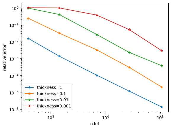
Plot error. We observe immense shear locking for polynomial order \(k=1\) as the pre-asymptotic regime increases rapidly. Increasing the polynomial order to \(k=2\) (or \(k=3\)) mitigates the problem, but it is still present.

import matplotlib.pyplot as plt

plt.yscale("log")
plt.xscale("log")
plt.xlabel("ndof")
plt.ylabel("relative error")
for i, result in enumerate(results):
    ndof, err = zip(*result)
    plt.plot(ndof, err, "-*", label="thickness=" + str(thicknesses[i]))
plt.legend()
plt.show()

8.4.2. TDNNS method

Next, we apply the TDNNS method to discretize the bending term \(\int_{\Omega}\| \varepsilon(\beta) \|_{\mathbb{D}}^2\) as in [Pechstein and Schöberl. The TDNNS method for Reissner-Mindlin plates. Numerische Mathematik 137, 3 (2017), 713-740].

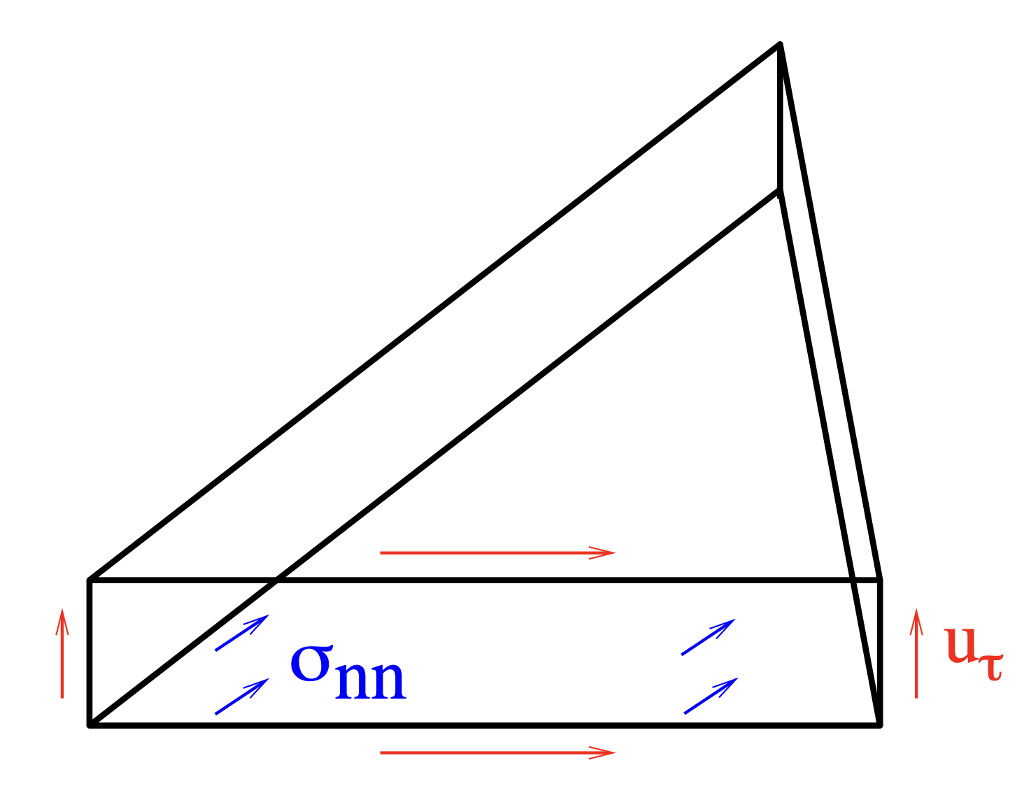
Instead of using Lagrangian elements, we discretize the rotations \(\beta\) in the Nedelec space. Thus, all discrete gradients \(\nabla w\) are in the space of rotations, and we don’t have the locking problem from before. By introducing the linearized bending moment tensor \(\sigma=\mathbb{D}\varepsilon(\beta)\) we obtain the following formulation.

Find \((\sigma,\beta, w) \in H(\mathrm{div} \mathrm{div})\times H(\mathrm{curl})\times H^1(\Omega)\) such that for all \((\tau,\delta, v) \in H(\mathrm{div} \mathrm{div})\times H(\mathrm{curl})\times H^1(\Omega)\)

\[\begin{align*} \begin{array}{ccccll} -\int_{\Omega} \mathbb{D}^{-1} \sigma : \tau\,dx & - & \left< \mathrm{div} \tau, \beta \right> & = & 0 \\ -\left< \mathrm{div} \sigma, \delta \right> & + & \frac{\kappa\, G}{t^2} \int_{\Omega} (\nabla w - \beta) (\nabla v - \delta)\,dx & = & \int_{\Omega} f v\,dx, \end{array} \end{align*}\]

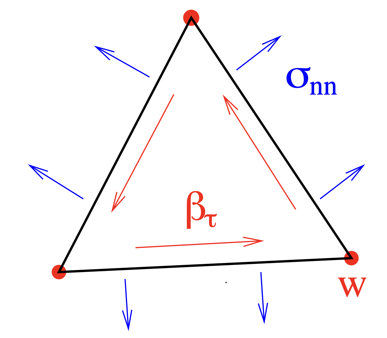
with the TDNNS duality pairing

\[\begin{align*} \langle \mathrm{div} \boldsymbol{\sigma}, \beta\rangle &= \sum_{T\in\mathcal{T}}\int_T\mathrm{div}\boldsymbol{\sigma}\cdot\beta\,dx -\int_{\partial T}\boldsymbol{\sigma}_{nt}\beta_t\,ds\\ &=-\sum_{T\in\mathcal{T}}\int_T\boldsymbol{\sigma}:\nabla \beta\,dx +\int_{\partial T}\boldsymbol{\sigma}_{nn}\beta_n\,ds =-\langle \boldsymbol{\sigma}, \nabla \beta\rangle \end{align*}\]

and the inverted elasticity tensor \(\mathbb{D}^{-1}\varepsilon = \frac{12(1-\nu^2)}{Et^3}\big(\frac{1}{1-\nu}\varepsilon-\frac{\nu}{1-\nu^2}\mathrm{tr}(\varepsilon)I_{2\times2}\big)\). Here \(\partial T\) denotes the element-boundary (edges) of \(T\), \(n\) the normal vector and \(t\) the tangential vector on \(\partial T\). With e.g. \(\sigma_{nt}:= t^\top\sigma n\) we denote the normal tangential component of \(\sigma\).

We use Lagrangian elements of order \(k\) for the displacement \(w\), and one order less for the rotations \(\beta\) and the bending moment tensor \(\sigma\).

def SolveReissnerMindlinTDNNS(mesh, order=1, thickness=0.1, draw=False):
    fesB = HCurl(mesh, order=order - 1, dirichlet="circ")
    fesS = HDivDiv(mesh, order=order - 1, dirichlet="")
    fesW = H1(mesh, order=order, dirichlet="circ")

    fes = fesW * fesB * fesS
    (w, beta, sigma), (v, delta, tau) = fes.TnT()

    n = specialcf.normal(2)

    a = BilinearForm(fes, symmetric=True)
    # bending part
    a += (
        -InnerProduct(DMatInv(sigma, E, nu), tau)
        + InnerProduct(tau, Grad(beta))
        + InnerProduct(sigma, Grad(delta))
    ) * dx
    a += -(sigma[n, n] * delta * n + tau[n, n] * beta * n) * dx(element_boundary=True)
    # shearing part
    a += k * G / thickness**2 * InnerProduct(Grad(w) - beta, Grad(v) - delta) * dx
    a.Assemble()

    f = LinearForm(fz * v * dx).Assemble()

    gf_solution = GridFunction(fes)
    gf_w, _, _ = gf_solution.components

    inv = a.mat.Inverse(fes.FreeDofs(), inverse="")
    gf_solution.vec.data = inv * f.vec
    if draw:
        Draw(gf_w, mesh, "w")

    return gf_w, fes

results = []

# try out polynomial order 1 and 2
order = 1

thicknesses = [1, 0.1, 0.01, 0.001]
with TaskManager():
    for t in thicknesses:
        results.append([])
        w_ex = ExactSolution(thickness=t)

        for i in range(5):
            mesh = GenerateMesh(order=order, maxh=0.5**i)
            gfw, fes = SolveReissnerMindlinTDNNS(
                mesh, order=order, thickness=t, draw=False
            )

            # relative L2-error of displacement
            err = sqrt(Integrate((gfw - w_ex) * (gfw - w_ex), mesh)) / sqrt(
                Integrate(w_ex * w_ex, mesh)
            )
            results[-1].append((fes.ndof, err))

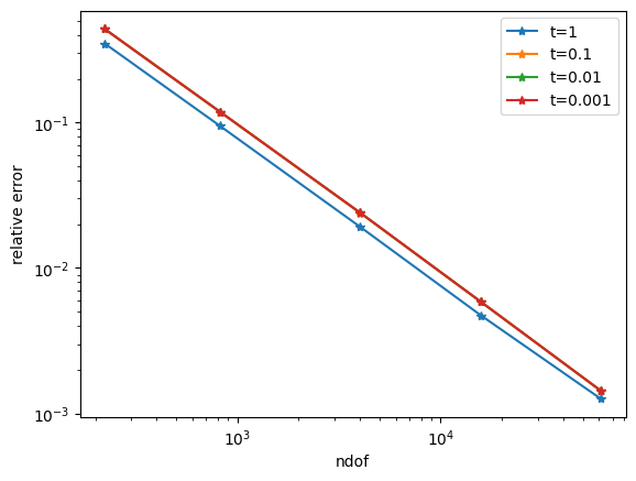
With the TDNNS method we obtain a locking free discretization already for polynomial degree \(k=1\) for the displacements.

import matplotlib.pyplot as plt

plt.yscale("log")
plt.xscale("log")
plt.xlabel("ndof")
plt.ylabel("relative error")
for i, result in enumerate(results):
    ndof, err = zip(*result)
    plt.plot(ndof, err, "-*", label="t=" + str(thicknesses[i]))
plt.legend()
plt.show()

In the limit \(t \to 0\) the shear energy term can be understood as a penalty formulation enforcing the Kirchhoff-Love assumption

\[\begin{align*} \beta = \nabla w. \end{align*}\]

Thus, in the limit case, the total energy simplifies by eliminating the rotation \(\beta\) to

\[\begin{align*} \mathcal{W}_{\mathrm{Kirchhoff-Love}}(w)=\frac{1}{2}\int_{\Omega}\| \varepsilon(\nabla w) \|_{\mathbb{D}}^2-\int_{\Omega}f\,w, \end{align*}\]

which is the Kirchhoff-Love plate model.

Drawback of the current implementation of the TDNNS formulation for Reissner-Mindlin plates: We have a mixed saddle point problem leading to an indefinite system matrix. This can be easily overcome with hybridization techniques NGSolve docu - Static condensation by breaking the normal-normal continuity of \(\sigma\) and reinforcing it by a Lagrange multiplier \(\alpha\). After static condensation a symmetric positive definite system is regained.

Exercise:

• Implement hybridization for TDNNS for Reissner-Mindlin plates