11.4. HDG Tricks (scalar)#

In this unit we want to discuss a few advanced tricks that can be used for further tuning of the \(H(\operatorname{div})\)-conforming Hybrid DG Stokes discretizations (and other 2nd order elliptic problems).

We want to treat:

  • projected jumps

  • 🫣 hidden dofs

  • Hybrid DG formulations based on lifting operators

For ease of discussion we will first start with a discussion of the first three features in the context of the Poisson problem

\[ - \Delta u = f \text{ in } \Omega, \quad u = g \text{ on } \partial \Omega \]

and will apply it directly afterwards to the Stokes problem.

Note

We will partially repeat the introduction of the projected jumps approach from the advanced tutorials here in order to provide a self-contained discussion and keep a consistent notation. Furthermore we will give more details on the tricks behind the curtain.

11.4.1. Preliminary: Recap of standard HDG #

The standard interior penalty DG method for the Poisson problem takes the form:

  • \(V_{h,g} = V_h^T \times \hat V_{h,g}\)

  • \(V_h^T = \mathbb{P}^{k}(\mathcal{T}_h)\) (discontinuous pol. on elements)

  • \(\hat V_h = \mathbb{P}^{k}(\mathcal{F}_h)\) (discontinuous pol. on facets), \(\hat V_{h,g} = \{\hat v \in \hat V_{h} \mid \hat v = \Pi^k g \text{ on } \partial \Omega\}\)

  • \(\underline{u}_h = (u_h,\hat u_h) \in V_{h,g}\) solves \(a_h(\underline{u}_h, \underline{v}_h) = f_h(\underline{v}_h)\) for all \(\underline{v}_{h} \in V_{h,0}\) with

    • HDG bilinear form \(a_h(\cdot,\cdot)\): \(\newline\displaystyle a_h(\underline{u}_h,\underline{v}_h) := \underbrace{\sum_{T \in \mathcal{T}_h} \int_T \nabla u \cdot \nabla v}_{=:b_h(u_h,v_h)} \underbrace{- \int_{\partial T} \nabla u \!\cdot \! n \cdot (v - \hat v)}_{=: N_h({u}_h,\underline{v}_h)} \underbrace{- \int_{\partial T} \nabla v \! \cdot \! n \cdot (u - \hat u)}_{= N_h({v}_h,\underline{u}_h)}\) \(\newline\displaystyle \hphantom{a_h(\underline{u}_h,\underline{v}_h) := }\underbrace{+ \frac{\gamma k^2}{h}\int_{\partial T} (u - \hat u) \cdot (v - \hat v)}_{=: S_h(\underline{u}_h,\underline{v}_h)},\)

    • HDG linear form \(f_h(\underline{v}_h)\): \( \newline\displaystyle f_h(\underline{v}_h) := \sum_{T \in \mathcal{T}_h} \int_T f v\).

Hide code cell source
# input : fes = V x Vhat:
def setup_HDG_system(fes, **opts):
    uh, vh = fes.TnT()
    (u,uhat), (v,vhat) = uh, vh
    jump = lambda uh: uh[0]-uh[1] 
    order = fes.components[0].globalorder
    alpha = 2
    h = specialcf.mesh_size
    n = specialcf.normal(mesh.dim)

    a = BilinearForm(fes, **opts)
    dS = dx(element_boundary=True)
    a += grad(u)*grad(v)*dx + \
        alpha*(order+1)**2/h*jump(uh)*jump(vh)*dS + \
        (-grad(u)*n*jump(vh) - grad(v)*n*jump(uh))*dS
    a.Assemble()
    
    f = LinearForm(fes)
    f += 5*v*dx
    f.Assemble()
    return a,f
Hide code cell source
def solve_lin_system(a,f,gfu,inverse=""):
    aSinv = a.mat.Inverse(gfu.space.FreeDofs(coupling=a.condense),inverse=inverse)
    if a.condense:
        ainv = ((IdentityMatrix(a.mat.height) + a.harmonic_extension) @ (aSinv + a.inner_solve) @ (IdentityMatrix(a.mat.height) + a.harmonic_extension_trans))        
    else:
        ainv = aSinv
    rhs = f.vec.CreateVector()
    rhs.data = f.vec - a.mat * gfu.vec
    gfu.vec.data += ainv * rhs
from ngsolve import *
from ngsolve.webgui import Draw
from netgen.occ import *

mesh = Mesh(unit_square.GenerateMesh(maxh=0.1))

order=1
V = L2(mesh, order=order)
F = FacetFESpace(mesh, order=order, dirichlet=".*")
fes = V*F

gfu = GridFunction(fes)
a,f, = setup_HDG_system(fes, condense=True)
solve_lin_system(a,f,gfu)

Draw (gfu.components[0], mesh, "u-HDG", deformation=True);

11.4.2. Projected Jumps (and how it works)#

An observation:

  • \(\nabla u \! \cdot \! n \in \mathcal{P}^{k-1}(F)\) on every facet \(F\),

  • hence \(N_h({u}_h,\underline{v}_h) = N_h({u}_h, \Pi_{\mathcal{F}_h}^{k-1} \underline{v}_h)\) where \(\Pi_{\mathcal{F}_h}^{k-1}\) is the \(L^2(\mathcal{F}_h)\) projection on \(\mathbb{P}^{k-1}(\mathcal{F}_h)\)

We then apply the following modifications:

  • To bound the \(N_h\)-terms it hence suffices to reduce the stabilizing term to \(S_h^{pj}(\cdot,\cdot) = S_h^{pj}(\Pi_{\mathcal{F}_h}^{k-1}(\cdot,\cdot))\)

  • We hence reduce the facet space to \(\hat V_h = \mathbb{P}^{k-1}(\mathcal{F}_h)\) (which reduces the globally coupled dofs, especially for low order methods)

Now the questions arises: How to realize the ``projected jumps’’ \(\Pi_{\mathcal{F}_h}^{k-1}(\mathcal{F}_h)\) in practice? One answer is discussed in the next section:

11.4.3. highest_order_dc: Highest order facet functions discontinuous#

The basis functions in \(\mathbb{P}^{\ell}(\mathcal{F}_h)\) ( corresponds to FacetFESpace(..., order=l, ...) in NGSolve) are constructed \(L^2\)-orthogonal (and order hierarchically).

The implementation trick for the ``projected jumps’’ method is to

  • use formally the same bilinear and linear form as in the standard HDG version,

  • but choose the following (seemingly more complicated) facet space:

\[ \hat V_h^\ast = \mathbb{P}^{k-1}(\mathcal{F}_h) \oplus \mathbb{P}^{k-1,\perp}(\partial \mathcal{T}_h) \]
sketch for highest order dc

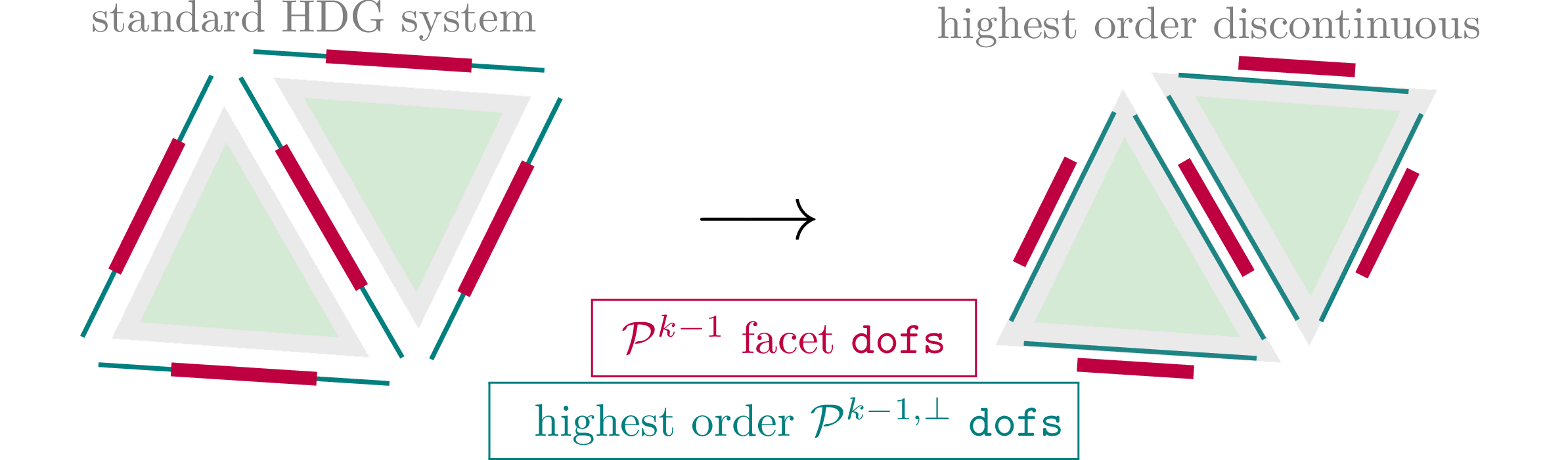
\(\hat V_h^\ast\) is to be read in the following way: Every function \(\hat v_h^\ast \in \hat V_h^\ast\) can be decomposed as \(\hat v_h^\ast = \hat v_h + \bar v_h\) where

  • on each facet \(F\) the \(\mathcal{P}^{k-1}(F)\)-part of the facet function, \(\hat v_h\), stays uni-valued while

  • the \(L^2\)-orthogonal complement in \(\mathbb{P}^{k}(F)\), \(\bar v_h\), becomes double-valued (one version for both aligned elements)

Testing with \((v_h, \hat v_h + \bar v_h) = (0,0,\bar v_h)\) with \(\bar v_h\) supported only on one facet \(F\) from one element side \(T\) in the discrete formulation we obtain only the part from the \(S_h(\cdot,\cdot)\) term (the other parts drop due to orthogonality):

\[ \frac{\gamma}{h} \int_F (u_h - \hat{u}_h - \bar u_h) \bar v_h = 0 \quad \forall \bar v_h \]

Hence, the element-local facet variable becomes

\[ \bar u_h = \Pi_{\mathcal{F}_h}^{k-1,\perp} (u_h - \hat u_h) \]

We can hence eliminate \(\bar u_h\) (in dependence of \(u_h\) and \(\hat u_h\)) from the equations. Plugging it in yields the projection as on every facet \(F\) (from one side of an element \(T\)) we have:

\[ u_h - \hat u_h - \bar u_h = (\operatorname{id} - \Pi_{\mathcal{F}_h}^{k-1,\perp} ) (u_h - \hat u_h) = \Pi_{\mathcal{F}_h}^{k-1} (u_h - \hat u_h) \]

So, in 2D we add one degree of freedom per edge:

Vhat = FacetFESpace(mesh, order=order, dirichlet=".*")
Vhats = FacetFESpace(mesh, order=order, dirichlet=".*", \
                          highest_order_dc=True)
print(f"Vhat.ndof = {Vhat.ndof}, Vhats.ndof = {Vhats.ndof}, difference = {Vhats.ndof - Vhat.ndof}, number of facets = {mesh.nfacet}")
Vhat.ndof = 718, Vhats.ndof = 1037, difference = 319, number of facets = 359

What is wrong? Make a guess!

The highest_order_dc-flag leaves boundary facets untouched!

Hide code cell source
print(f"boundary facets: {mesh.GetNE(BND)}")
boundary facets: 40

We have introduced more unknowns, but

  • the new unknowns stay element-local and can be condensed out

print(f"Vhat.nfreedofs = {sum(Vhat.FreeDofs(coupling=True))}, Vhats.nfreedofs = {sum(Vhats.FreeDofs(coupling=True))}")
Vhat.nfreedofs = 638, Vhats.nfreedofs = 319

11.4.4. 🫣HIDDEN_DOFs#

We actually do not care about \(\bar u_h\). Can’t we get rid of it in the FESpace (to get problems of smaller dimension)?

Yes! In NGSolve we have a type of degrees of freedom that we denote as HIDDEN_DOF. These need to fulfill the following three requirements:

  1. the degree of freedom only appears on one element

  2. the degree of freedom is only needed during assembly, not reconstruction of the dof necessary afterwards

  3. the r.h.s. of the linear system for that dof is zero

All three requirements are fulfilled for the highest order dofs after setting highest_order_dc on:

  1. The dofs are element-local (only one side of a facet see it)

  2. The dof only realizes the \(L^2\)-projection, we don’t need it afterwards

  3. Above we have exploited exactly that the r.h.s. is zero for \(\bar v_h\).

There are two places where HIDDEN_DOFs play a role:

  1. when setting up linear systems and the sparsity plays a role (depending on the flags condense and eliminate_hidden of the corresonding BilinearForm)

  2. when reducing the size of an FESpace using the Wrapper space Compress

  3. reduces the number of matrix entries, 2. reduces the dimension of vectors and matrices.

Warning

Note that you can do 1. without considering 2. but not 2. without 1., i.e. without adjusting your linear systems

Vhats2 = FacetFESpace(mesh, order=order, dirichlet=".*", \
                            highest_order_dc=True, \
                            hide_highest_order_dc=True)
Vhats3 = Compress(Vhats2)
print(f"  Vhat.ndof = {Vhat.ndof}, \n Vhats.ndof = {Vhats.ndof}, \nVhats2.ndof = {Vhats2.ndof}, \nVhats3.ndof = {Vhats3.ndof}")
  Vhat.ndof = 718, 
 Vhats.ndof = 1037, 
Vhats2.ndof = 1037, 
Vhats3.ndof = 359

So, to get the most out of the situation we need three components here:

  • ⛓️‍💥 highest_order_dc=True to split the highest order function(s) to the aligned elements and make them local LOCAL_DOFs

  • 🫣 hide_highest_order_dc=True to have these dofs not only LOCAL_DOFs but even HIDDEN_DOFs

  • 🗜️ Compress(...) to really eliminate them from the global space (actually Compress is a wrapper space)

Lets take a look at the local and global numbering and COUPLING_TYPEs on one element:

spaces = [Vhat,Vhats,Vhats2,Vhats3]
print("l.dof|  std. FacetFES |+highest_o..._dc|+hide_highest_..|     + Compress |" )
print("-----|----------------|----------------|----------------|----------------|" )
for els in zip(*[V.Elements() for V in spaces]):
    for ldof, gdofs in enumerate(zip(*[el.dofs for el in els])):
        print(f"{ldof:3}->|",end="")
        for i, gdof in enumerate(gdofs):
            if gdof >= 0:
                print(f" {gdof:4}:{str(spaces[i].CouplingType(gdof)).removeprefix('COUPLING_TYPE.').removesuffix('_DOF'):10}",end="|")
            else:
                print("  ---:----------", end="|")
        print("")
    break
l.dof|  std. FacetFES |+highest_o..._dc|+hide_highest_..|     + Compress |
-----|----------------|----------------|----------------|----------------|
  0->|    2:WIREBASKET|    1:WIREBASKET|    1:WIREBASKET|    1:WIREBASKET|
  1->|    3:INTERFACE |  359:LOCAL     |  359:HIDDEN    |  ---:----------|
  2->|   22:WIREBASKET|   11:WIREBASKET|   11:WIREBASKET|   11:WIREBASKET|
  3->|   23:INTERFACE |  360:LOCAL     |  360:HIDDEN    |  ---:----------|
  4->|    0:WIREBASKET|    0:WIREBASKET|    0:WIREBASKET|    0:WIREBASKET|
  5->|    1:INTERFACE |  361:LOCAL     |  361:HIDDEN    |  ---:----------|

Let’s apply the different versions to solve the PDE problem:

order=1
V = L2(mesh, order=order)
defopt = {"mesh":mesh, "order":order, "dirichlet":".*"}
facfes = [(FacetFESpace(**defopt),"FacFES"), \
          (FacetFESpace(**defopt, highest_order_dc=True),"FacFES+ho_dc"), \
          (FacetFESpace(**defopt, highest_order_dc=True, hide_highest_order_dc=True),"FacFES+ho_dc+hide"), \
          (Compress(FacetFESpace(**defopt, highest_order_dc=True, hide_highest_order_dc=True)),"FacFES+ho_dc+hide+compr.")]
gfuT_vis = GridFunction(V, multidim=True)
for i, (F,fstring) in enumerate(facfes):
    fes = V*F
    gfu = GridFunction(fes)
    a,f, = setup_HDG_system(fes, condense=True)
    solve_lin_system(a,f,gfu)
    if i == 0:
        gfuT_vis.vec.data = gfu.components[0].vec
    else:
        gfuT_vis.AddMultiDimComponent(gfu.components[0].vec)  
    print(f"{fstring:25}", end="")
    print(f"ndofs:{fes.ndof:5}({V.ndof:5}+{F.ndof:5}), ",end="")
    print(f"n.coup.dofs:{sum(fes.FreeDofs(coupling=True)):5}, ", end=""),
    print(f"non-zeros:{a.mat.nze:8}")
Draw (gfuT_vis, mesh, "u", deformation=True);
FacFES                   ndofs: 1396(  678+  718), n.coup.dofs:  638, non-zeros:    6860
FacFES+ho_dc             ndofs: 1715(  678+ 1037), n.coup.dofs:  319, non-zeros:    1715
FacFES+ho_dc+hide        ndofs: 1715(  678+ 1037), n.coup.dofs:  319, non-zeros:    1715
FacFES+ho_dc+hide+compr. ndofs: 1037(  678+  359), n.coup.dofs:  319, non-zeros:    1715

What happens during static condensation with HIDDEN_DOFs?

When calculating an element matrix, we obtain a matrix that can be partitioned according to three categories:

  • I: INTERFACE_DOFs (including WIREBASKET_DOFs): Degrees of freedom that couple locally

  • L: LOCAL_DOFs: Degrees of freedom that only couple with other degrees of freedom within the element, but not outside

  • H: HIDDEN_DOFs: Degrees of freedom that also do not couple element-locally and meet the above conditions.

\[\begin{align*} \begin{pmatrix} A_{II} & A_{IL} & A_{IH} \\ A_{LI} & A_{LL} & A_{LH} \\ A_{HI} & A_{HL} & A_{HH} \end{pmatrix} \end{align*}\]

Now we know that the right-hand side with respect to the H-rows vanishes and that no further contributions will arise outside the element for the H-rows and H-columns during the assembly process.

\[\begin{split} \begin{pmatrix} A_{II} & A_{IL} & A_{IH} \\ A_{LI} & A_{LL} & A_{LH} \\ A_{HI} & A_{HL} & A_{HH} \end{pmatrix} \begin{pmatrix} u_I \\ u_L \\ u_H \end{pmatrix} = \begin{pmatrix} \\ \\ 0 \end{pmatrix} \end{split}\]

We assume that \(A_{HH}\) is invertible and that we can form the Schur complement. The Schur complement \( \tilde A \) of matrix \( A \) w.r.t. \( A_{HH} \) is:

\[\begin{split} \begin{pmatrix} \tilde A_{II} & \tilde A_{IL} \\ \tilde A_{LI} & \tilde A_{LL} \end{pmatrix} = \begin{pmatrix} A_{II} & A_{IL} \\ A_{LI} & A_{LL} \end{pmatrix} - \begin{pmatrix} A_{IH} \\ A_{LH} \end{pmatrix} A_{HH}^{-1} \begin{pmatrix} A_{HI} & A_{HL} \end{pmatrix} \end{split}\]

After the Schur complement is formed, we can directly forget about \(u_H\) and the matrix entries of the HIDDEN_DOFs on that element. Next, we can form the Schur complement w.r.t. \(\tilde A_{LL}\) if we want, cf. the unit on static condensation in NGSolve.

Overall, there are three options on how to treat the HIDDEN_DOF and LOCAL_DOFs when setting up linear systems:

  • condense=True: Static condensation is applied to the HIDDEN_DOFs and LOCAL_DOFs:

    • LOCAL_DOFs still appear in the factors of the “harmonic ext.”,

    • but the global system is solved only for the INTERFACE_DOFs.

    • HIDDEN_DOFs are removed after the first Schur complement step and don’t appear in the matrix

  • eliminate_hidden=True:

    • HIDDEN_DOFs are removed with the first Schur complement step, but no further static condensation is applied.

    • LOCAL_DOFs are treated in the same way as INTERFACE_DOFs (except for preconditioning where WIREBASKET_DOFs are still distinguished)

  • eliminate_hidden=False (default) and condense=True (default):

    • No Schur complement is formed at all.

Hide code cell source
linsys_opts = [({"condense": False},"  none"), \
               ({"eliminate_hidden": True},"hidden"), \
               ({"condense": True}," local")]
for i, (F,fstring) in enumerate(facfes):
    print(fstring)
    for j, (opts,elims) in enumerate(linsys_opts):
        print(f"condensed dofs: "+elims+", ",end="")
        fes = V*F
        a,f, = setup_HDG_system(fes, **opts)
        print(f"ndofs:{fes.ndof:5}({V.ndof:5}+{F.ndof:5}), ",end="")
        print(f"n.coup.dofs:{sum(fes.FreeDofs(coupling=True)):5}, ", end=""),
        print(f"non-zeros:{a.mat.nze:8}")
    print("")
FacFES
condensed dofs:   none, ndofs: 1396(  678+  718), n.coup.dofs:  638, non-zeros:   17030
condensed dofs: hidden, ndofs: 1396(  678+  718), n.coup.dofs:  638, non-zeros:   17030
condensed dofs:  local, ndofs: 1396(  678+  718), n.coup.dofs:  638, non-zeros:    6860

FacFES+ho_dc
condensed dofs:   none, 
ndofs: 1715(  678+ 1037), n.coup.dofs:  319, non-zeros:   17987
condensed dofs: hidden, ndofs: 1715(  678+ 1037), n.coup.dofs:  319, non-zeros:   17987
condensed dofs:  local, 
ndofs: 1715(  678+ 1037), n.coup.dofs:  319, non-zeros:    1715

FacFES+ho_dc+hide
condensed dofs:   none, ndofs: 1715(  678+ 1037), n.coup.dofs:  319, non-zeros:   17987
condensed dofs: hidden, 
ndofs: 1715(  678+ 1037), n.coup.dofs:  319, non-zeros:    7817
condensed dofs:  local, 
ndofs: 1715(  678+ 1037), n.coup.dofs:  319, non-zeros:    1715

FacFES+ho_dc+hide+compr.
condensed dofs:   none, 
ndofs: 1037(  678+  359), n.coup.dofs:  319, non-zeros:    7817
condensed dofs: hidden, ndofs: 1037(  678+  359), n.coup.dofs:  319, non-zeros:    7817
condensed dofs:  local, ndofs: 1037(  678+  359), n.coup.dofs:  319, non-zeros:    1715

11.4.5. HDG Lifting’s#

As a next application of HIDDEN_DOFs we consider the lifting operator approach for the DG discretization.

The stability term \(S_h(\cdot,\cdot)\) in the HDG bilinear form makes up for the \(N_h(\cdot,\cdot)\)-parts that include the normal gradient on the element boundary. To obtain a more fine-grained control over this term, we can introduce a lifting operator that allows us to rewrite the stabilization term in a more flexible way:

The HDG lifting operator \(\mathcal{L}: \mathbb{P}^k(\mathcal{T}_h) \times \mathbb{P}^k(\mathcal{F}_h) \to \mathbb{P}^{k}(\mathcal{T}_h)\) is defined for \(\underline{v}_h \in V_h = V_h^T \times \hat V_h\) so that

\[ b_h(\mathcal{L}(\underline{v}_h), w_h) + \underbrace{\sum_T \int_T h^{-2} \Pi^0 \mathcal{L}(\underline{v}_h) \Pi^0 w_h }_{=:j_h(\mathcal{L}(\underline{u}_h),w_h)}= N_h(w_h,\underline{v}_h) \quad \forall w_h \in \mathbb{P}^{k}(\mathcal{T}_h). \]

Note that with \(w_h = w_h^0 + w_h^\perp\) and \(N_h(w_h^0, \cdot) = b_h(\cdot, w_h^) = 0\) we obtain \(\Pi^0 \mathcal{L}(\underline{v}_h) = 0\) and hence

\[ b_h(\mathcal{L}(\underline{v}_h), w_h) = N_h(w_h,\underline{v}_h). \]

With this we obtain:

\[\begin{align*} a_h(\underline{u}_h,\underline{v}_h) := & b_h(u_h,v_h) + b_h(\mathcal{L}(\underline{v}_h),u_h) + b_h(\mathcal{L}(\underline{u}_h),v_h) \\ & + S_h(\mathcal{L}(\underline{u}_h),\mathcal{L}(\underline{v}_h)) \\ =& b_h(u_h + \mathcal{L}(\underline{u}_h), v_h + \mathcal{L}(\underline{v}_h)) \\ & + S_h(\mathcal{L}(\underline{u}_h),\mathcal{L}(\underline{v}_h)) - b_h(\mathcal{L}(\underline{u}_h),\mathcal{L}(\underline{v}_h)) \end{align*}\]

Now, it is easy to see, that new sufficient stabilizations (without need for a sufficiently large parameter) can be designed easily.

We simply take

\[ S_h(\mathcal{L}(\underline{u}_h),\mathcal{L}(\underline{v}_h)) = b_h(\mathcal{L}(\underline{u}_h),\mathcal{L}(\underline{v}_h)) + \underbrace{\frac{\gamma k}{h}\int_{\partial T} (u - \hat u) \cdot (v - \hat v)}_{=:s_h(\underline{u}_h,\underline{v}_h)} \]

Note that the latter part makes it definite. Otherwise even multiples of the former part my not be sufficient if the lifting operator has a non-trivial kernel (due to a non-trivial kernel of \(N_h(\cdot,\cdot)\)), which can easily happen. Further note that the penalty term is scaled with \(\gamma k/h\) instead of \(\gamma k^2/h\) and \(\gamma > 0\) is all we need to ask for (no “sufficiently large”).

This yields

\[ a_h(\underline{u}_h,\underline{v}_h) := b_h(u_h,v_h) + b_h(\mathcal{L}(\underline{v}_h),u_h) + b_h(\mathcal{L}(\underline{u}_h),v_h) + 2 b_h(\mathcal{L}(\underline{u}_h),\mathcal{L}(\underline{v}_h)) \]

Now, for the implementation we rewrite the terms using the lifting characteristics backwards:

\[\begin{align*} \tag{A} a_h(\underline{u}_h,\underline{v}_h) & := b_h(u_h,v_h) + N_h(u_h,\underline{v}_h) + N_h(v_h,\underline{u}_h) + N_h(\mathcal{L}(\underline{u}_h),\underline{v}_h) + s_h(\underline{u}_h,\underline{v}_h) \end{align*}\]

To implement the second-last part we introduce a new variable \(u_h^\ell = \mathcal{L}(\underline{u}_h)\) for which the lifting equality holds:

\[\begin{align*} \tag{B} - b_h(u_h^\ell, v_h^\ell) - j_h(u_h^\ell, v_h^\ell) + N_h(v_h^\ell,\underline{u}_h) = 0 \quad \forall v_h^\ell \in \mathbb{P}^{k,-0}(\mathcal{T}_h). \end{align*}\]

Now, Plugging \(u_h^\ell = \mathcal{L}(\underline{u}_h)\) into (A) and adding (B) yields the new formulation: Find \(\underline{\underline{u}}_h = (\underline{u}_h, u_h^\ell) \in V_h \times \mathbb{P}^{k}(\mathcal{T}_h)\) so that

\[\begin{align*} a_h(\underline{\underline{u}}_h,\underline{\underline{v}}_h) & := b_h(u_h,v_h) + N_h(u_h,\underline{v}_h) + N_h(v_h,\underline{u}_h) + s_h(\underline{u}_h,\underline{v}_h) \\ & \qquad + N_h(u_h^\ell,\underline{v}_h) + N_h(v_h^\ell,\underline{u}_h) \\ & \qquad - b_h(u_h^\ell, v_h^\ell) - j_h(u_h^\ell, v_h^\ell) \\ & = f_h(\underline{v}_h) \qquad \qquad \forall \underline{\underline{v}}_h = (\underline{v}_h, u_h^\ell) \in V_h \times \mathbb{P}^{k,-0}(\mathcal{T}_h). \end{align*}\]
def setup_lifted_HDG_system(fes, **opts):
    uh, vh = fes.TnT()
    order = fes.components[0].globalorder
    (u,uhat,ul), (v,vhat,vl) = uh, vh
    jump = lambda uh: uh[0]-uh[1] 
    h = specialcf.mesh_size
    n = specialcf.normal(mesh.dim)
    a = BilinearForm(fes, **opts)
    dS = dx(element_boundary=True)
    a += grad(u)*grad(v)*dx # b_h
    a += (-grad(u)*n*jump(vh) - grad(v)*n*jump(uh))*dS #N_h
    a += 1*(order+1)/h*jump(uh)*jump(vh)*dS # s_h
    a += -grad(ul)*grad(vl)*dx # b_h (lifting)
    a += (-grad(ul)*n*jump(vh) - grad(vl)*n*jump(uh))*dS #N_h (lifting)
    a += - 1/(h*h)* ul * vl * dx(bonus_intorder=-2*order) # j_h
    a.Assemble()
    
    f = LinearForm(fes)
    f += 5*v*dx
    f.Assemble()
    return a,f

We note that the new variable \(u_h^\ell\) can be treated as HIDDEN variable as

  • it only appears on one element

  • it is only needed during assembly (to realize the lifting)

  • the r.h.s. of the linear system for \(v_h^\ell\) is zero

We use the keyword hide_all_dofs to make all dofs in a space HIDDEN:

order=1
V = L2(mesh, order=order)
F = FacetFESpace(mesh, order=order, dirichlet=".*")
#F = Compress(FacetFESpace(mesh, order=order, dirichlet=".*", highest_order_dc=True, hide_highest_order_dc=True))
Vl = Compress(L2(mesh, order=order, hide_all_dofs=True))
fes = V*F*Vl

Is Vl empty now?

Yes and no:

print(f"global ndof: {Vl.ndof}")

for el in Vl.Elements():
    print(f"local dofs on first element: {el.dofs}")
    break
global ndof: 0
local dofs on first element: [-2, -2, -2]

Warning

Setting dofs as HIDDEN_DOFs changes the global number of dofs and the global numbering (after compression), but on the element level the number of dofs is unaffected! The computation of the element matrix (before applying Schur complement strategies) is independent of any information on coupling types in the FESpace.

gfuT_vis = GridFunction(V, multidim=True)
gfu = GridFunction(fes)
for i, (opt, elims) in enumerate(reversed(linsys_opts)): 
    a,f, = setup_lifted_HDG_system(fes, **opt)
    solve_lin_system(a,f,gfu)
    print(f"condensed dofs: {elims:6}, nzes: {a.mat.nze}")    
    if i == 0:
        gfuT_vis.vec.data = gfu.components[0].vec
    else:
        gfuT_vis.AddMultiDimComponent(gfu.components[0].vec)  
Draw (gfuT_vis, mesh, "u-HDG", deformation=True);
condensed dofs:  local, nzes: 6860
condensed dofs: hidden, nzes: 17030
condensed dofs:   none, nzes: 17030

Warning

Recall: Don’t use HIDDEN_DOFs + Compress without setting condense=True or eliminate_hidden=True in the BilinearForm!

Note

Also here for the chosen lifting formulation we don’t need to penalize jumps up to order \(k\) to have a proper norm. Instead we can use the “projected jumps” approach. To try it out comment in/out the corresponding lines for Vhat above.