4.4. Hybrid Discontinuous Galerkin methods#
use additionally the hybrid facet variable on the skeleton:
the jump-term is now replaced by the difference \(u - \widehat u\).
No additional matrix entries across elements are produced. Dirichlet boundary conditions are set as usual to the facet variable:
from ngsolve import *
from ngsolve.webgui import Draw
from netgen.occ import *

def AtomicShape(maxh = 0.1):
    ax2d = gp_Ax2d(gp_Pnt2d(0.5, 0.5), gp_Dir2d(1, 0))
    outeli = Ellipse( ax2d, 0.5, 0.1)
    ineli = Ellipse( ax2d, 0.3, 0.06)

    shape = outeli.Face() - ineli.Face()


    shape += shape.Rotate(gp_Ax1(gp_Pnt(0.5, 0.5, 0), gp_Dir(0,0,1)), 120)
    shape += shape.Rotate(gp_Ax1(gp_Pnt(0.5, 0.5, 0), gp_Dir(0,0,1)), 240)
    shape += Circle((0.5,0.5),0.2).Face()

    Draw(shape)
    geo = OCCGeometry(shape, dim = 2)
    return Mesh(geo.GenerateMesh(maxh = maxh)).Curve(3)

mesh = AtomicShape()
order=2
V = L2(mesh, order=order)
F = FacetFESpace(mesh, order=order, dirichlet=".*")
fes = V*F
u,uhat = fes.TrialFunction()
v,vhat = fes.TestFunction()
Now, the jump is the difference between element-term and facet-term:
jump_u = u-uhat
jump_v = v-vhat
r_centr = (x-0.5)**2+(y-0.5)**2

f = LinearForm(100*exp(10*r_centr)*v*dx).Assemble()
alpha = 4
condense = False
h = specialcf.mesh_size
n = specialcf.normal(mesh.dim)

a = BilinearForm(fes, condense=condense)
dS = dx(element_boundary=True)
a += grad(u)*grad(v)*dx + \
    alpha*order**2/h*jump_u*jump_v*dS + \
    (-grad(u)*n*jump_v - grad(v)*n*jump_u)*dS

b = CF( (20,1) )
uup = IfPos(b*n, u, uhat)
a += -b * u * grad(v)*dx + b*n*uup*jump_v *dS
a.Assemble()

#f = LinearForm(1*v*dx).Assemble()

gfu = GridFunction(fes)

print ("A non-zero elements:", a.mat.nze)
A non-zero elements: 181395
if not condense:
    inv = a.mat.Inverse(fes.FreeDofs(), "pardiso")
    gfu.vec.data = inv * f.vec
else:
    fmod = (f.vec + a.harmonic_extension_trans * f.vec).Evaluate()

    inv = a.mat.Inverse(fes.FreeDofs(True), "pardiso")
    gfu.vec.data = inv * fmod

    gfu.vec.data += a.harmonic_extension * gfu.vec
    gfu.vec.data += a.inner_solve * f.vec

Draw (gfu.components[0], mesh, "u-HDG");
4.4.1. Remarks on sparsity pattern in NGSolve#
import scipy.sparse as sp
import matplotlib.pylab as plt
A = sp.csr_matrix(a.mat.CSR())
plt.spy(A, markersize=2)
<matplotlib.lines.Line2D at 0x7fbfbf8e4ed0>
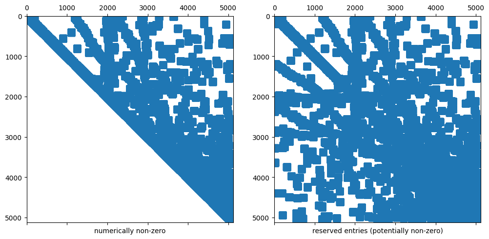
4.4.1.1. Remark 1: The sparsity pattern is set up a-priorily#
The sparsity pattern of a sparse matrix in NGSolve is independent of its entries (it’s set up a-priorily).
We can have “nonzero” entries that have the value 0
Below we show the reserved memory for the sparse matrix and the (numerically) non-zero entries in this sparse matrix.
fes2 = L2(mesh, order=order, dgjumps=True)
u,v=fes2.TnT()
a3 = BilinearForm(fes2)
a3 += u*v*dx + (u+u.Other())*v*dx(skeleton=True)
a3.Assemble();
import scipy.sparse as sp
import matplotlib.pylab as plt
plt.rcParams['figure.figsize'] = (12, 12)
A = sp.csr_matrix(a3.mat.CSR())
fig = plt.figure(); ax1 = fig.add_subplot(121); ax2 = fig.add_subplot(122)
ax1.set_xlabel("numerically non-zero"); ax1.spy(A)
ax2.set_xlabel("reserved entries (potentially non-zero)"); ax2.spy(A,precision=-1)
plt.show()
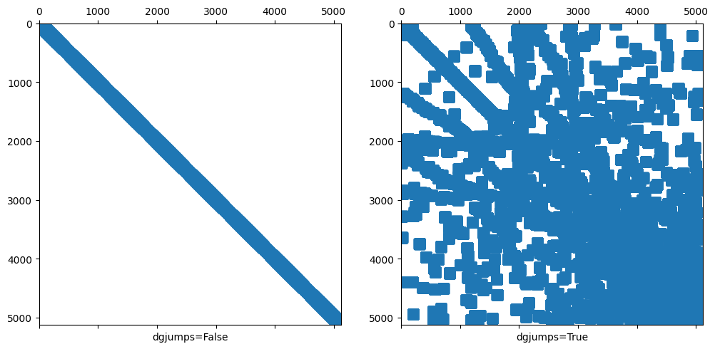
4.4.1.2. Remark 2: Sparsity pattern with and without dgjumps=True is different#
a1 = BilinearForm(L2(mesh, order=order, dgjumps=False)); a1.Assemble()
a2 = BilinearForm(L2(mesh, order=order, dgjumps=True)); a2.Assemble()
A1 = sp.csr_matrix(a1.mat.CSR())
A2 = sp.csr_matrix(a2.mat.CSR())
fig = plt.figure(); ax1 = fig.add_subplot(121); ax2 = fig.add_subplot(122)
ax1.set_xlabel("dgjumps=False"); ax1.spy(A1,precision=-1)
ax2.set_xlabel("dgjumps=True"); ax2.spy(A2,precision=-1)
plt.show()
used dof inconsistency
(silence this warning by setting BilinearForm(...check_unused=False) )
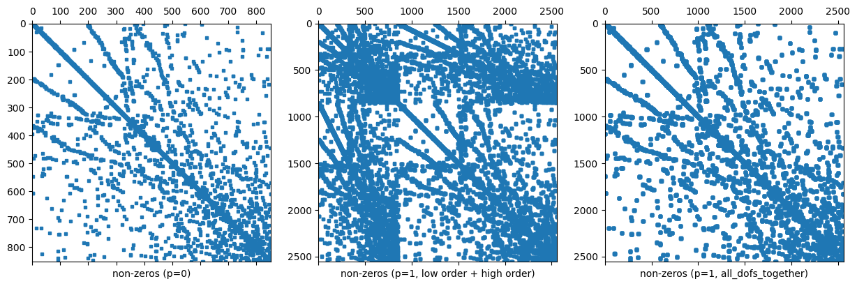
4.4.1.3. Remark 3: Dof numbering of higher order FESpaces#
In
NGSolveFESpaces typically have a numbering where the first block of dofs corresponds to a low order subspace (which is convenient for iterative solvers).For L2 this means that the first dofs correspond to the constants on elements.
You can turn this behavior off for some spaces, e.g. for L2 by adding the flag
all_dofs_together.
We demonstrate this in the next comparison:
plt.rcParams['figure.figsize'] = (15, 15)
fig = plt.figure()
ax = [fig.add_subplot(131), fig.add_subplot(132), fig.add_subplot(133)]

for i, (order, all_dofs_together, label) in enumerate([(0,False, "non-zeros (p=0)"),
                                                    (1,False,"non-zeros (p=1, low order + high order)"),
                                                    (1,True,"non-zeros (p=1, all_dofs_together)")]):
    a = BilinearForm(L2(mesh,order=order,dgjumps=True,all_dofs_together=all_dofs_together))
    a.Assemble()
    ax[i].spy(sp.csr_matrix(a.mat.CSR()),markersize=3,precision=-1)
    ax[i].set_xlabel(label)