from netgen.occ import *
from ngsolve import *
from ngsolve.webgui import Draw
import numpy as np
from newtonmethod import NewtonWithLinesearch
import matplotlib.pyplot as plt
import ipywidgets as widgets

SetNumThreads(4)
9.4. A buckling problem#
A toroidal panel is subjected to a vertical body load. At one end, the panel is simply supported; as the load is increased, buckling is observed.
See also: Vetyukov, Y. (2014). Nonlinear mechanics of thin-walled structures: asymptotics, direct approach and numerical analysis. Springer Science & Business Media.
ea = { "euler_angles" : [-45,1,-4] }


thickness = 0.001
RAD = 1.5
RAD2 = 0.5
E, nu = 2.1e11, 0.3
rho = 7800

mu = E/2/(1-nu)
lam = E*nu/(1+nu)/(1-2*nu)

sqrt2 = np.sqrt(2)
arc1 = ArcOfCircle(Pnt(RAD,0,-RAD2), Pnt(RAD+RAD2/sqrt2,0,-RAD2/sqrt2), Pnt(RAD+RAD2,0,0))
arc2 = ArcOfCircle(Pnt(RAD+RAD2,0,0), Pnt(RAD+RAD2/sqrt2,0,RAD2/sqrt2), Pnt(RAD,0,RAD2))

seg = Wire([arc1,arc2])

face = seg.Revolve(Axis((0,0,0),Z),90).bc("mat")

geo = OCCGeometry(face)

ngmesh = geo.GenerateMesh(maxh=RAD2/2)
mesh = Mesh(ngmesh)

ngmesh.SetCD2Name(1, "bottom")
ngmesh.SetCD2Name(2, "internal")
ngmesh.SetCD2Name(3, "rightbottom")
ngmesh.SetCD2Name(4, "leftbottom")
ngmesh.SetCD2Name(5, "top")
ngmesh.SetCD2Name(6, "righttop")
ngmesh.SetCD2Name(7, "lefttop")
mesh = Mesh(ngmesh)

order = 3
mesh.Curve(order)

scene = Draw(mesh, **ea)
9.4.1. Problem setup#
A Kirchhoff-Love shell formulation is used to model the panel. Let \(\mathbf A\) and \(\mathbf B\) be the first and second metric tensor, meaning \(\mathbf A\) is the projection onto the tangential plane, and \(\mathbf B = - \nabla_S \vec N\) the negative gradient of the surface normal. The model is described kinematically using midsurface displacement \(\vec u\), the surface deformation gradient \(\mathbf F_S = \mathbf A + \nabla_S \vec u\), membrane strains \(\mathbf{e}\) and curvature \(\boldsymbol{\kappa}\), for details see the according shell tutorial. We use a shell energy for St.Venant-Kirchhoff materials, amounting to
For static load \(\rho g\, \vec e_z\) in the shell’s associated volume, the problem amounts to solving
9.4.1.1. Load stepping and buckling#
Additionally to the degrees of freedom necessary for the shell formulation, two Lagrangian multipliers are added: the first one being the load factor \(g\) scaling the contribution \(\rho g\), the second the mean normal displacement of the shell in vertical direction (thus the dual of the load). Note that setting \(g=9.81 m/s^2\) corresponds to gravity, however in this example also higher load factors are considered.
For the initial mesh above, the buckling mode cannot be represented even at polynomial order \(k=3\). Therefore, an adaptive scheme is considered, where the load factor is raised up to \(g=50\) in load steps.
9.4.1.2. ZZ error estimate for shells#
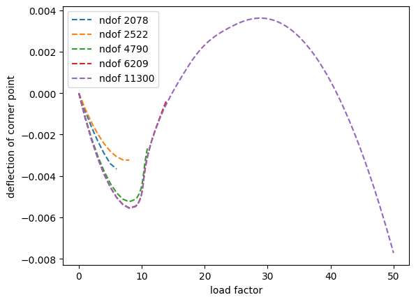
In each load step, an error estimate of Zienkiewicz-Zhu type for the bending moments is computed. If no convergence is reached, or if the error estimate reaches some critical value, adaptive mesh refinement based the error estimate is performed. After some cycles, the computation is satisfactory. The deflection of a corner point of the panel is monitored.
BCclamp = ""
BCfix = "left.*"
fes1 = HDivDivSurface(mesh, order=order-1, discontinuous=True)
fes2 = VectorH1(mesh, order=order, dirichlet_bbnd=BCfix)
fes3 = HDivSurface(mesh, order=order-1, orderinner=0, dirichlet_bbnd=BCclamp)
fes4 = HCurlCurl(mesh, order=order-1, discontinuous=True)
fes5 = FESpace("number", mesh)
fes  = fes2*fes1*fes3*fes4*fes4*fes4*fes5*fes5
u_, mom_, hyb_, eps_, R_, kappa_, p_, umean_ = fes.TrialFunction()
mom_, hyb_, eps_, R_, kappa_ = mom_.Trace(), hyb_.Trace(), eps_.Trace(), R_.Operator("dualbnd"), kappa_.Trace()


fesVF = VectorFacetSurface(mesh, order=order)
b_ = fesVF.TrialFunction()
b_.Reshape((3,))

fesF = FacetSurface(mesh, order=0)

solution = GridFunction(fes, name="solution")
solution_0 = GridFunction(fes)
averednv = GridFunction(fesVF)
averednv_start = GridFunction(fesVF)


u, mom, hyb, eps, R, kappa, p, umean = solution.components
glist = np.concatenate((\
    np.linspace(0,9,10),
    np.linspace(9,11,21),
    np.linspace(11,50,2*39+1))
)


loadsteplists = []
uzlists = []
umeanlists = []
ndoflist = []


maxndof = 10000
ndof_coupling = sum(fes.FreeDofs(True))
refstep = 0
while ndof_coupling < maxndof:

    loadsteplists.append([])
    uzlists.append([])
    umeanlists.append([])

    fes.Update()
    fesVF.Update()
    fesF.Update()
    solution.Update()
    solution_0.Update()
    averednv.Update()
    averednv_start.Update()
    ndof_coupling = sum(fes.FreeDofs(True))

    ndoflist.append(ndof_coupling)

    par = Parameter(0.0)


    nsurf = specialcf.normal(mesh.dim)
    t     = specialcf.tangential(mesh.dim)
    nel   = Cross(nsurf, t)

    A    = Id(mesh.dim) - OuterProduct(nsurf,nsurf)
    Ftau    = grad(u_).Trace() + A
    Ctau    = Ftau.trans*Ftau
    Etautau = 0.5*(Ctau - A)

    nphys   = Normalize(Cof(Ftau)*nsurf)
    tphys   = Normalize(Ftau*t)
    nelphys = Cross(nphys,tphys)

    Hn = CoefficientFunction( (u_.Operator("hesseboundary").trans*nphys), dims=(3,3) )

    cfnphys = Normalize(Cof(A+grad(solution.components[0]))*nsurf)

    cfn  = Normalize(CoefficientFunction( averednv.components ))
    cfnR = Normalize(CoefficientFunction( averednv_start.components ))
    pnaverage = Normalize( cfn - (tphys*cfn)*tphys )


    averednv.Set(nsurf, dual=True, definedon=mesh.Boundaries(".*"))
    averednv_start.vec.data = averednv.vec

    gradn = specialcf.Weingarten(3) #grad(nsurf)


    bfA = BilinearForm(fes, symmetric=True, condense=True)


    A1 = E*thickness*nu/(1-nu*nu)
    A2 = E*thickness/(1+nu)
    D1 = thickness**2/12*A1
    D2 = thickness**2/12*A2
    bfA += Variation(0.5*(A1*Trace(eps_)**2 + A2*InnerProduct(eps_,eps_))*ds).Compile()
    bfA += Variation(0.5*(D1*Trace(kappa_)**2 + D2*InnerProduct(kappa_,kappa_))*ds).Compile()

    bfA += Variation( (InnerProduct(mom_, kappa_ + Hn + (1-nphys*nsurf)*gradn))*ds ).Compile()
    bfA += Variation( InnerProduct(eps_-Etautau, R_)*ds(element_vb=BND) )
    bfA += Variation( InnerProduct(eps_-Etautau, R_)*ds(element_vb=VOL) )
    bfA += Variation( -(acos(nel*cfnR)-acos(nelphys*pnaverage)-hyb_*nel)*(mom_*nel)*nel*ds(element_boundary=True) ).Compile()

    bfA += Variation( u_[2]*rho*thickness*(p_)*ds )
    bfA += Variation( (par-p_)*rho*thickness*umean_*ds)


    Vmtilde = H1(mesh, order=order)**9
    mtilde = GridFunction(Vmtilde)

    scene = Draw(Norm(mom), mesh, "absm", deformation=u, **ea)
    loadwidget = widgets.Text(value="g = 0")
    display(loadwidget)


    with TaskManager():
        for gg in glist:# in range(0,numsteps):
            solution_0.vec.data = solution.vec
            par.Set(gg)

            averednv.Set(nsurf, dual=True, definedon=mesh.Boundaries(".*"))


            newtonerr, numit = NewtonWithLinesearch(a=bfA, x=solution.vec, abserror=1e-7, maxnewton=15)

            if newtonerr:
                break

            uz = (solution.components[0])(mesh(RAD, 0, -RAD2,BND))[2]

            uzlists[-1] += [uz]
            umeanlists[-1] += [solution.components[-1].vec[0]]
            loadsteplists[-1] += [gg]

            scene.Redraw()
            loadwidget.value = f"g = {gg}"

            mtilde.Set(mom, definedon=mesh.Boundaries(".*"))


            err = sqrt(InnerProduct(mom-mtilde,mom-mtilde))

            eta2 = Integrate(err, mesh, BND, element_wise=True)

            maxerr = max(eta2)
            if maxerr > 5e-2: break

    print(f"Using {ndof_coupling} coupling dofs, simulation up to load factor g = {loadsteplists[-1][-1]}")

    if (ndof_coupling < maxndof):

        for el in mesh.Elements(BND):
            mesh.SetRefinementFlag(el, eta2[el.nr] > 0.25*maxerr)


        mesh.Refine(True)
        mesh.Curve(order)

    refstep += 1
Using 2078 coupling dofs, simulation up to load factor g = 6.0
Newton did not converge
Using 2522 coupling dofs, simulation up to load factor g = 8.0
Newton did not converge
Using 4790 coupling dofs, simulation up to load factor g = 10.9
Newton did not converge
Using 6209 coupling dofs, simulation up to load factor g = 14.0
Using 11300 coupling dofs, simulation up to load factor g = 50.0
for i in range(len(uzlists)):
    uzlist = uzlists[i]
    loadlist = loadsteplists[i]
    plt.plot(loadlist, uzlist, "--", label = f"ndof {ndoflist[i]}")

plt.legend()
plt.xlabel("load factor")
plt.ylabel("deflection of corner point")
Text(0, 0.5, 'deflection of corner point')