4.3. Discontinuous Galerkin Methods

• Use discontinuous finite element spaces to solve PDEs.

• Allows upwind-stabilization for convection-dominated problems

• Requires additional jump terms for consistency

Interior penalty DG form for \(-\Delta u\):

\[ A(u,v) = \sum_T \int_T \nabla u \nabla v - \sum_F \int_F \{ n \nabla u \} [v] - \sum_F \int_F \{ n \nabla v \} [u] + \frac{\alpha p^2}{h} \sum_F \int_F [u][v] \]

with jump-term over facets: $\( [u] = u_{left} - u_{right} \)$

and averaging operator $\( \{ n \nabla u \} = \tfrac{1}{2} (n_{left} \nabla u_{left} + n_{left} \nabla u_{right}) \)$

DG form for \(\text{div} (b u)\), where \(b\) is the given wind:

\[ B(u,v) = -\sum_T b u \nabla v + \sum_F \int_F b\cdot n u^{upwind} v \]

from ngsolve import *
from ngsolve.webgui import Draw
from netgen.occ import *

def AtomicShape(maxh = 0.1):
    ax2d = gp_Ax2d(gp_Pnt2d(0.5, 0.5), gp_Dir2d(1, 0))
    outeli = Ellipse( ax2d, 0.5, 0.1)
    ineli = Ellipse( ax2d, 0.3, 0.06)

    shape = outeli.Face() - ineli.Face() 


    shape += shape.Rotate(gp_Ax1(gp_Pnt(0.5, 0.5, 0), gp_Dir(0,0,1)), 120)
    shape += shape.Rotate(gp_Ax1(gp_Pnt(0.5, 0.5, 0), gp_Dir(0,0,1)), 240)
    shape += Circle((0.5,0.5),0.2).Face() 

    Draw(shape)
    geo = OCCGeometry(shape, dim = 2)
    return Mesh(geo.GenerateMesh(maxh = maxh)).Curve(3)

mesh = AtomicShape()

The space is responsible for allocating the matrix graph. Tell it that it should reserve entries for the coupling terms:

order=2
fes = L2(mesh, order=order, dgjumps=True)
u,v = fes.TnT()

Every facet has a master element. The value from the other element is referred to via the Other() operator:

jump_u = u-u.Other()
jump_v = v-v.Other()
n = specialcf.normal(2)
mean_dudn = 0.5*n * (grad(u)+grad(u.Other()))
mean_dvdn = 0.5*n * (grad(v)+grad(v.Other()))

Integrals on facets are computed by setting skeleton=True.

• dx(skeleton=True) iterates over all internal faces

• ds(skeleton=True) iterates over all boundary faces

alpha = 4
h = specialcf.mesh_size
diffusion = grad(u)*grad(v) * dx \
    +alpha*order**2/h*jump_u*jump_v * dx(skeleton=True) \
    +(-mean_dudn*jump_v-mean_dvdn*jump_u) * dx(skeleton=True) \
    +alpha*order**2/h*u*v * ds(skeleton=True) \
    +(-n*grad(u)*v-n*grad(v)*u)* ds(skeleton=True)

a = BilinearForm(diffusion).Assemble()

r_centr = (x-0.5)**2+(y-0.5)**2

f = LinearForm(100*exp(10*r_centr)*v*dx).Assemble()

gfu = GridFunction(fes, name="uDG")
gfu.vec.data = a.mat.Inverse() * f.vec
Draw (gfu);

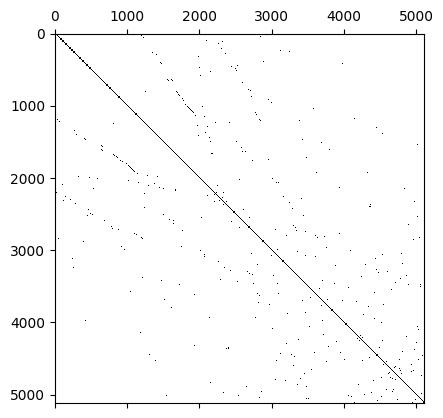
DG requires a lot of additional matrix entries:

fes2 = L2(mesh, order=order)
ul2,vl2 = fes2.TnT()
a2 = BilinearForm(ul2*vl2*dx).Assemble()
print ("DG-matrix nze:", a.mat.nze)
print ("L2-matrix nze:", a2.mat.nze)

DG-matrix nze: 114948
L2-matrix nze: 30708

Let’s see why: we plot the sparsity pattern of the matrix.

import scipy.sparse as sp
import matplotlib.pylab as plt
A = sp.csr_matrix(a.mat.CSR())
plt.spy(A, markersize=0.1)

<matplotlib.lines.Line2D at 0x7fb2c0163690>

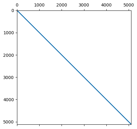
and here the sparsity pattern of the matrix in \(L^2\), you can notice that the elements cannot exchange information with their neighbors.

import matplotlib.pyplot as plt
A2 = sp.csr_matrix(a2.mat.CSR())
plt.spy(A2, markersize=0.1)

<matplotlib.lines.Line2D at 0x7fb2c01c1810>

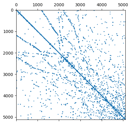
Next we are solving a convection-diffusion problem:

alpha = 4
h = specialcf.mesh_size

The IfPos checks whether the first argument is positive. Then it returns the second one, else the third one. This is used to define the upwind flux. The check is performed in every integration-point on the skeleton:

b = CF( (20,5) )
uup = IfPos(b*n, u, u.Other())

convection = -b * u * grad(v)*dx + b*n*uup*jump_v * dx(skeleton=True)

acd = BilinearForm(diffusion + convection).Assemble()

gfu = GridFunction(fes)
gfu.vec.data = acd.mat.Inverse(freedofs=fes.FreeDofs(),inverse="pardiso") * f.vec
Draw (gfu)

BaseWebGuiScene

import matplotlib.pyplot as plt
Acd = acd.mat.ToDense()
plt.spy(Acd)

<matplotlib.image.AxesImage at 0x7fb2c0192cd0>