8.2. Timoschenko and Euler-Bernoulli beam

In this section we consider the Timoschenko and Euler-Bernoulli beam equations. If we have a structure \(\Omega\subset\mathbb{R}^2\) where one dimension is significantly thinner than the other a dimension reduction to a one-dimensional problem can be done. For example, \(\Omega = (0,1)\times (-t/2,t/2)\) to the midsurface \(\mathcal{S}=(0,1)\). For the (linear) elasticity problem on \(\Omega\) the Timoschenko and Euler-Bernoulli beam are two frequently used models. We start with the Timoschenko beam.

8.2.1. Timoschenko beam

The Timoschenko beam includes the vertical deflection of the beam and rotational degrees of freedom. The corresponding energy reads

\[\begin{align*} \mathcal{W}(u,\beta) = \int_0^1\Big(\frac{E}{24}|\beta^\prime|^2 + \frac{\kappa G}{2t^2}|u^\prime-\beta|^2\Big)\,dx - \int_0^1u\,f\,dx, \end{align*}\]

where the first term corresponds to the bending energy of the beam (\(\beta^\prime=u^{\prime\prime}\) is the linearized curvature of the beam) and the second is the shear energy measuring the deviation of the rotation \(\beta\) to the linearized rotated normal vector of the beam. Here, \(\kappa=5/6\) and \(G=E/(2(1+\nu))\) denote the shear correction factor and shearing modulus, respectively, and \(E\) is the Young’s modulus.

We clamp the left side of the beam and define \(H^1_{\Gamma}((0,1))=\{v\in H^1((0,1))\,\vert\, v(0)=0\}\).

By taking the variations of the energy we obtain the problem: For given force \(f\) find \((u,\beta)\in H^1_{\Gamma}((0,1))\times H^1_{\Gamma}((0,1))\) such that for all \((\delta u,\delta\beta)\in H^1_{\Gamma}((0,1))\times H^1_{\Gamma}((0,1))\)

\[\begin{align*} \int_0^1\frac{E}{12}\beta^\prime(\delta\beta)^\prime\,dx + \frac{\kappa G}{t^2}\int_0^1(u^\prime-\beta)((\delta u)^\prime-\delta\beta)\,dx = \int_0^1\delta u\,f\,dx. \end{align*}\]

A straight forward discretization approach is to use Lagrangian finite elements of the same order for the displacement and rotation \(u_h,\beta_h\in V_h^k\times V_h^k\), which is known to induce locking for small thickness parameters \(t\). In the limit \(t\to 0\) the shearing energy can be seen as a penalty enforcing \(u_h^\prime=\beta_h\). In the lowest order case this equation forces the piecewise constant \(u^\prime_h\) to fit with the linear and continuous \(\beta_h\) leading to the trivial solution, \(u_h=0\). This situation is called shear locking. The constants in Cea’s Lemma are not uniform in the thickness parameter. One can show that if the mesh size \(h\) is of the order of the thickness \(t\), the correct convergence rates start. From the theory of mixed methods we know that inserting on \(L^2\)-projection into the shearing term cures this problem be relaxing the constraint. In 1D this is equivalent to a numerical under-integration using only the mid-point rule for the shearing term. One can also proof that for at least quadratic order \(k=2\) no shear locking occurs for the Timoschenko beam. (Note, that this is not true for plates.)

from ngsolve import *
from ngsolve.meshes import Make1DMesh
from ngsolve.webgui import Draw

mu, lam = 0.5, 0  # Lame parameter
nu = lam / (2 * (lam + mu))  # Possion ratio (=0)
E = mu * (3 * lam + 2 * mu) / (lam + mu)  # Young's modulus (=1)
G = E / (2 * (1 + nu))  # shearing modulus
k = 5 / 6  # shear correction factor

def SolveTimoschenkoBeam(order, mesh, thickness, reduced_integration=False, draw=False):
    V = H1(mesh, order=order, dirichlet="left")
    fes = V * V
    (u, beta), (du, dbeta) = fes.TnT()

    a = BilinearForm(fes, symmetric=True)
    a += E / 12 * grad(beta) * grad(dbeta) * dx + k * G / thickness**2 * (
        grad(u) - beta
    ) * (grad(du) - dbeta) * dx(bonus_intorder=-reduced_integration)
    a.Assemble()

    f = LinearForm(-0.1 * du * ds("right")).Assemble()

    gf_solution = GridFunction(fes)
    gf_w, gf_beta = gf_solution.components

    gf_solution.vec.data = a.mat.Inverse(fes.FreeDofs(), inverse="") * f.vec

    if draw:
        Draw(gf_w, mesh, deformation=CF((0, gf_w, 0)), min=0, max=0)

    return gf_w(mesh(1, 0, 0)), gf_w, gf_beta


SolveTimoschenkoBeam(order=2, mesh=Make1DMesh(10), thickness=0.01, draw=True);

Test for different thicknesses the convergence for a sequence of refined meshes.

Try out reduced integration or setting the polynomial order to \(k=2\).

thicknesses = [10 ** (-i) for i in range(1, 5)]
results = []
with TaskManager():
    for t in thicknesses:
        results.append([])
        for num_el in [2**i for i in range(1, 9)]:
            displacement, _, _ = SolveTimoschenkoBeam(
                order=1, mesh=Make1DMesh(num_el), thickness=t, reduced_integration=False
            )
            results[-1].append((num_el, displacement))

Plot the deflections. We observe for \(k=1\) and no reduced integration that a pre-asymptotic regime rapidly increases, where the displacement solution is zero. Using reduced integration with \(k=1\) cures the problem. Also increasing the polynomial degree to \(k=2\) (or higher) overcomes the shear locking (also without reduced integration).

import matplotlib.pyplot as plt

plt.yscale("linear")
plt.xscale("log")
plt.xlabel("number of elements")
plt.ylabel("displacement")
for i, result in enumerate(results):
    num_el, displacement = zip(*result)
    plt.plot(num_el, displacement, label=f"thickness={thicknesses[i]}")
plt.legend()
plt.show()

for i in range(len(results)):
    print(f"tip deflection for thickness {thicknesses[i]} = {results[i][-1][1]}")

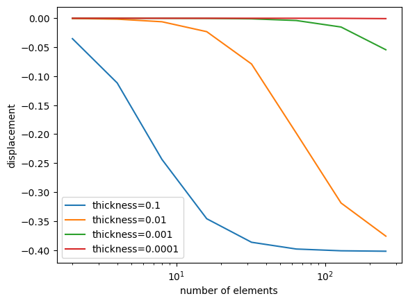
tip deflection for thickness 0.1 = -0.4021443235277204
tip deflection for thickness 0.01 = -0.37611147630787406
tip deflection for thickness 0.001 = -0.05436389621147861
tip deflection for thickness 0.0001 = -0.0006281575957822956

8.2.2. Euler-Bernoulli beam

In the limit \(t\to0\) the equality \(u^\prime=\beta\) is forced to hold. Therefore, the rotation \(\beta\) has to coincide with the linearized normal vector of the deformed beam \(u^\prime\) and can be eliminated from the equation.

This gives the Euler-Bernoulli beam: For given force \(f\) find \(u\in H^2_{\Gamma}((0,1))=\{v\in H^2((0,1))\,\vert\, v(0)=v^\prime(0)=0\}\) such that for all \(\delta u\in H^2_{\Gamma}((0,1))\)

\[\begin{align*} \int_0^1\frac{E}{12}u^{\prime\prime}(\delta u)^{\prime\prime}\,dx = \int_0^1\delta u\,f\,dx. \end{align*}\]

Note that the thickness parameter \(t\) does not enter the equation anymore. Therefore it is locking-free, but \(C^1\)-conforming finite elements are required as it is now a fourth order problem now.

Let’s rewrite it as a mixed saddle-point problem by introducing the bending \(\sigma=\frac{E}{12}u^{\prime\prime}\) as additional unknown

\[\begin{align*} &\int_{0}^{1} \frac{12}{E}\sigma\delta\sigma\,dx -\int_{0}^{1}u^{\prime\prime}\delta\sigma\,dx &&= 0, &&\quad \forall \delta\sigma,\\ &-\int_{0}^{1}\sigma(\delta u)^{\prime\prime}\,dx &&= -\int_0^1 \delta u\,f \,dx, &&\quad \forall \delta u, \end{align*}\]

and use integration by parts such that it is well defined for \(u,\sigma\in H^1(0,1)\)

\[\begin{align*} &\int_{0}^{1} \frac{12}{E}\sigma\delta\sigma\,dx +\int_{0}^{1}u^{\prime}(\delta\sigma)^\prime\,dx &&= 0,\\ &\int_{0}^{1}\sigma^\prime(\delta u)^{\prime}\,dx &&= -\int_0^1 \delta u\,f \,dx. \end{align*}\]

For prescribing clamped boundary conditions we use essential Dirichlet data for the dispalcement, \(u=0\), but homogeneous Neumann data for \(\sigma\). \(\sigma=0\) would physically mean that the stress is applied which cooresponds to free boundary conditions. Therefore we set \(\sigma=0\) at the free boundary. This swap of boundary condition is classical for mixed problems.

def SolveEulerBernoulliBeam(order, mesh, draw=True):
    fes = H1(mesh, order=order, dirichlet="left") * H1(
        mesh, order=order, dirichlet="right"
    )
    (u, sigma), (du, dsigma) = fes.TnT()
    force = -0.1

    a = BilinearForm(fes, symmetric=True)
    a += (
        12 / E * sigma * dsigma + grad(u) * grad(dsigma) + grad(du) * grad(sigma)
    ) * dx
    a.Assemble()

    f = LinearForm(-force * du * ds("right")).Assemble()

    gf_solution = GridFunction(fes)

    gf_solution.vec.data = a.mat.Inverse(fes.FreeDofs(), inverse="") * f.vec
    gf_u, gf_sigma = gf_solution.components

    if draw:
        Draw(gf_u, mesh, deformation=CF((0, gf_u, 0)), min=0, max=0)
    return gf_u(mesh(1, 0, 0))


print(SolveEulerBernoulliBeam(order=2, mesh=Make1DMesh(100), draw=True))

-0.3999999999999487