17. Nankai Through with Heterogeneous Material

A preconditioner for the Helmholtz equation

\[\begin{alignat*}{2} -\Delta u - \kappa^2 u &= 0 \quad && \text{ in } \Omega, \\ \nabla u \cdot \mathbf{n} + j \kappa u &= g \quad && \text{ on } \partial \Omega \end{alignat*}\]

is introduced. It is based upon the mixed hybrid Discontinous Galerkin (HDG) formulation introduced in Hybridizing Raviart-Thomas Elements for the Helmholtz Equation. For the HDG formulation static condensation is emploid and for the resulting system of linear equations on the skeleton, a block Jacobi Preconditioner is applied. For more information about the formulation in combination with iterative solver strategies see Hybrid discontinuous Galerkin methods for the wave equation.

17.1. Geometry

As geometry a slice of the Nankai trough is used. It consists of a cube, but the used varying velocity field in the formulation makes the example very interesting. The data for the velocity field is contributed by A. Górszczyk and S. Operto. GO_3D_OBS: the multi-parameter benchmark geomodel for seismic imaging method assessment and next-generation 3D survey design (version 1.0). The problem is excited by a Gauß-peak from above.

from netgen.occ import *
from ngsolve import *
from ngsolve.webgui import Draw
import numpy as np

scalingfactor = 2.5
p = 4
k = 2*pi*4 *scalingfactor
maxh = 5 / scalingfactor

transbnd = "transparent"
excbnd = transbnd

xl = 20; yl = 102; zl = 28.3
x0 = 10; y0 = 12.5; z0 = 0; sg = 5
r2 = (x-x0)**2 + (y-y0)**2 + (z-z0)**2
excitation = exp(-r2/sg)

cube = Box((0,0,0), (xl,yl,zl))
cube.faces.name=transbnd
mesh = Mesh(OCCGeometry(cube).GenerateMesh(maxh=maxh))

17.2. Initialising the Velocity

The velocity data for the simulation is either loaded from the local disc or downloaded if it does not exist already.

from pathlib import Path
nankaiMatFile = Path("nankaiMat.bin")
if not nankaiMatFile.is_file():
    url = "https://www.geoazur.fr/WIND/pub/nfs/FWI-DATA/GEOMODELS/GO_3D_OBS/TARGET_PAPERS/v.bin"
    import os
    print("download velocity data")
    os.system("curl " + url + " --output nankaiMat.bin")
    print("download complete")

#load material from file
mat = np.fromfile("nankaiMat.bin", dtype = np.float32)
n1=284; n2=1021; n3=201
mat = mat.reshape((n3,n2,n1))
mat = mat.astype(complex)
mat = mat.transpose()
ccoef = VoxelCoefficient((0,0,0), (xl, yl, zl), mat)
matcoeff = 1/ccoef
sqrtmatcoeff = sqrt(matcoeff)
Draw(ccoef, mesh, "material", draw_surf=True, draw_vol=False, order=2, euler_angles=[120,1,-79]);

17.3. Weak Formulation

The mixed formulation is stated on the space \(L_2(\Omega) \times H_{pw}(div, \Omega) \times L_2(\mathcal{F}) \times L_2(\mathcal{F})\) with the sesquilinearform

\[\begin{alignat*}{2} s(u, \sigma, \hat u, \hat \sigma; v, \tau, \hat v, \hat \tau) := \sum_{T \in \mathcal{T}} &\int_T j\kappa \sqrt{M} u v - div(\sigma) v - u div(\tau) - j \kappa \sigma \tau d\mathbf{x} + \int_{\partial T} \sigma \cdot \mathbf{n} \hat v + \hat u \tau \cdot \mathbf{n} d \mathbf{s} \\ + &\int_{\partial T} \frac{2}{\sqrt{M}}(\sigma - \hat \sigma) \cdot \mathbf{n} (\tau - \hat \tau) \cdot \mathbf{n} - \frac{\sqrt{M}}{2}(\Pi^p u - \hat u) (\Pi^p v - \hat v) d\mathbf{s} - \int_{\partial \Omega} \sqrt{M} \hat u \hat v d \mathbf{s} \end{alignat*}\]

and the physical material coefficient \(M\).

In the sesquilinearform condensation is enabled and internal elements matrices are not stored to reduce the memory consumption. This implies that at the end the solution need to be extended from skeleton unknowns onto elements. The method of projected jumps by Schöberl and Lehrenfeld is applied to increase the polynomial order of the scalar variable \(u\) on elements.

U = L2(mesh, order=p+1, complex=True)
V = Discontinuous(HDiv(mesh, order=p, complex=True, RT=True)) # P^k Sub RT Sub P^k+1, div(RT) = P^k
FD = FacetFESpace(mesh, order=p+1, complex=True, highest_order_dc = True)
FN = NormalFacetFESpace(mesh, order=p, complex=True)
X = U*V*FD*FN
print("nDof:", X.ndof, "(u", U.ndof, ", sigma", V.ndof, ", uhat", FD.ndof, ", sigmahat", FN.ndof, ")")
    
(u,sigma,uh,sigman), (v,tau,vh,taun) = X.TnT()

a = BilinearForm(X, eliminate_internal=True, keep_internal=False)
n = specialcf.normal(mesh.dim)
dS = dx(element_boundary=True)

alpha = 1/2*sqrtmatcoeff
beta = 1/alpha
a += (1j*k*matcoeff*u*v - 1j*k*sigma*tau - div(sigma)*v - u*div(tau)) * dx
a += (sigma*n*vh + tau*n*uh + beta*(sigma-sigman)*n*(tau-taun)*n - alpha*(u-uh)*(v-vh)) * dS
a += - sqrtmatcoeff * uh.Trace()*vh.Trace() * ds(transbnd)
    
f = LinearForm(X)
f += excitation * vh.Trace() * ds(excbnd)

nDof: 7126260 (u 1514520 , sigma 3245400 , uhat 1507710 , sigmahat 858630 )

17.4. Skeleton Block Jacobi Preconditioner in 3D

The unknowns on a face are combined into a block for the block Jacobi preconditioner.

def GenerateBlocks3D(ablf, mesh, X):
    freedofs = X.FreeDofs()
    blocks = []
    for facet in mesh.facets:
        vdofs = []
        facedofs = X.GetDofNrs(facet)
        for fdof in facedofs:
            if freedofs[fdof]:
                vdofs.append(fdof)
        blocks.append(vdofs)
    return blocks

gfu = GridFunction(X)
with TaskManager():
    print("Assemble a")
    a.Assemble()
    print("Assemble f")
    f.Assemble()
    blocks = GenerateBlocks3D(a, mesh, X)
    pre = a.mat.CreateBlockSmoother(blocks, GS=False)
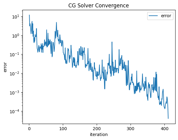
    solvers.CG(mat=a.mat, rhs=f.vec, sol=gfu.vec, pre=pre, maxsteps=1500, tol=1e-5, plotrates=True)
    print("Compute internal solution")
    a.ComputeInternal (gfu.vec, f.vec)
    print("Done")

Compute internal solution

Done

<Figure size 640x480 with 0 Axes>

Draw(gfu.components[2], mesh, "pressure", min=-1e-1, max=1e-1, \
     draw_surf=True, draw_vol=False, order=2, animate_complex=True, euler_angles=[120,1,-79]);