Nonlinear Koiter and Naghdi Shells via Hellan-Herrmann-Johnson and TDNNS

9.3. Nonlinear Koiter and Naghdi Shells via Hellan-Herrmann-Johnson and TDNNS#

In this section we solve the nonlinear Koiter and Naghdi shell equations with the HHJ and TDNNS method. Three examples are presented, where the second involves a structure with kinks and branched shells.

9.3.1. Nonlinear Koiter shell with HHJ#

9.3.1.1. Discretization method#

We start with the following three-field formulation [Neunteufel, Schöberl: The Hellan-Herrmann-Johnson and TDNNS method for linear and nonlinear shell, arXiv (2023).] to incorporate the distributional extrinsic curvature difference of the initial and deformed shell configuration:

Find $(u, κ^{diff}, σ) \in V_{h}^{k} \times M_{h}^{k - 1, dc} \times M_{h}^{k - 1}$ for the Lagrangian

\begin{aligned} L (u, κ^{diff}, σ) & = \int_{S} (\frac{t}{2} ‖ E_{S} (u) ‖_{M}^{2} + \frac{t^{3}}{12} ‖ κ^{diff} ‖_{M}^{2}) d s + \sum_{T \in T} \int_{T} (κ^{diff} - (F_{S}^{T} \nabla_{S} (ν \circ ϕ) - \nabla_{S} \hat{ν})) : σ d s \\ + \sum_{E \in E} \int_{E} (∢ (ν_{L} \circ ϕ, ν_{R} \circ ϕ) - ∢ ({\hat{ν}}_{L}, {\hat{ν}}_{R})) σ_{\hat{μ} \hat{μ}} d l - \int_{S} f \cdot u d s . \end{aligned}

Here, $E_{S} = \frac{1}{2} (F_{S}^{⊤} F_{S} - P_{S}) = \frac{1}{2} (\nabla_{S} u^{⊤} \nabla_{S} u + \nabla_{S} u^{⊤} P_{S} + P_{S} \nabla_{S} u)$ denotes the Green-strain tensor restricting on the tangent space measuring the membrane energy of the shell, $t$ the thickness, and $M$ the material tensor. $ν$ and $\hat{ν}$ are the normal vectors with respect to the deformed and initial configuration, respectively. $\hat{μ}$ is the co-normal (element-normal) vector.

With this formulation we circumvented the fourth order problem by means of a mixed one and are able to compute the bending energy also on affine triangulations thanks to the edge terms measuring the angle difference between the initial and deformed configuration.

For an invertible material law, we can eliminate $κ^{diff}$ leading to a mixed saddle point problem in the displacement $u$ and moment tensor $σ$ . The term $F_{S}^{T} \nabla_{S} (ν \circ ϕ) - \nabla_{S} \hat{ν}$ can be rewritten and simplified. The following formulation can be seen as an extension of the Hellan-Herrmann-Johnson method from linear plates to nonlinear shells [Neunteufel, Schöberl: The Hellan-Herrmann-Johnson method for nonlinear shell, Comput. Struct. (2019).].

Find $(u, σ) \in V_{h}^{k} \times M_{h}^{k - 1}$ for the Lagrangian

\begin{aligned} L (u, σ) & = \int_{S} (\frac{t}{2} ‖ E_{S} (u) ‖_{M}^{2} - \frac{6}{t^{3}} ‖ σ ‖_{M^{- 1}}^{2}) d s + \sum_{T \in T} \int_{T} σ : (H_{ν \circ ϕ} + (1 - \hat{ν} \cdot ν \circ ϕ) \nabla_{S} \hat{ν}) d s \\ + \sum_{E \in E} \int_{E} (∢ (ν_{L} \circ ϕ, ν_{R} \circ ϕ) - ∢ ({\hat{ν}}_{L}, {\hat{ν}}_{R})) σ_{\hat{μ} \hat{μ}} d l - \int_{S} f \cdot u d s, \end{aligned}

where $H_{ν \circ ϕ} = \sum_{i = 1}^{3} (\nabla_{S}^{2} u_{i}) ν_{i} \circ ϕ$ , and $\nabla_{S}^{2} u_{i} = P_{S} \nabla_{S} (\nabla_{S} u_{i})$ denotes the Riemann surface Hessian.

9.3.1.2. Cylindrical shell under volume load#

As a first example we consider a cylindrical shell, which is clamped at the left side and free at the right side, and applying a volume force.

from netgen.occ import *
from ngsolve import *
from ngsolve.webgui import Draw
import ipywidgets as widgets

order = 4

cyl = Cylinder((0, 0, 0), (1, 0, 0), 0.4, 1).faces[0]
cyl.edges.Min(X).name = "left"
cyl.edges.Min(X).hpref = 1
cyl.edges.Max(X).name = "right"
mesh = Mesh(OCCGeometry(cyl).GenerateMesh(maxh=0.1)).Curve(order)
mesh.RefineHP(2, 0.3)
mesh.Curve(order)
Draw(mesh, euler_angles=[0, -50, -10])

E, nu = 2e1, 0.1
thickness = 0.02

At the clamped boundary we need to fix the displacement by homogeneous Dirichlet boundary conditions. As usual for mixed formulations the essential and natural boundary conditions swap for the stress field. Therefore, we have to set the essential boundary condition $σ_{\hat{μ} \hat{μ}}$ at the free boundary. $σ_{\hat{μ} \hat{μ}} = 0$ has the physical meaning that no moment-force is applied at this boundary.

fes1 = HDivDivSurface(mesh, order=order - 1, dirichlet_bbnd="right")
fes2 = VectorH1(mesh, order=order, dirichlet_bbnd="left")
fes = fes2 * fes1
u, sigma = fes.TrialFunction()
# need the trace as we are on a surface
sigma = sigma.Trace()

fesRegge = HCurlCurl(mesh, order=order - 1)

gf_solution = GridFunction(fes, name="solution")

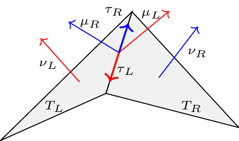
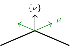
We define the unit normal vector $\hat{ν}$ , edge-tangential vector $\hat{t}$ and the co-normal vector $\hat{μ} = \hat{ν} \times \hat{t}$ at the initial configuration.

Then the projection operator onto the tangent space, deformation gradient, Cauchy-Green, and Green tensors $P_{S}$ , $F_{S}$ , $C_{S}$ , and $E_{S}$ are introduced.

Finally, the unit normal, edge-tangential, and co-normal vectors $ν, τ, μ$ on the deformed configuration are declared, which depend on the unknown displacement field $u$ .

# Surface unit normal, edge-tangential, and co-normal vectors on initial configuration
nv = specialcf.normal(mesh.dim)
tv = specialcf.tangential(mesh.dim)
cnv = Cross(nv, tv)

# Projection to the surface tangent space
Ptau = Id(mesh.dim) - OuterProduct(nv, nv)
Ftau = Grad(u).Trace() + Ptau
Etautau = 0.5 * (Ftau.trans * Ftau - Ptau)

# Surface unit normal, edge-tangential, and co-normal vectors on deformed configuration
nv_def = Normalize(Cof(Ftau) * nv)
tv_def = Normalize(Ftau * tv)
cnv_def = Cross(nv_def, tv_def)

# Surface Hessian weighted with unit normal vector on deformed configuration
H_nv_def = (u.Operator("hesseboundary").trans * nv_def).Reshape((3, 3))

For the angle computation of the bending energy we use an averaged unit normal vector avoiding the necessity of using information of two neighbored element at once (+ a more stable formulation using the co-normal vector instead of the unit normal vector)

\begin{aligned} \sum_{E \in E} \int_{E} (∢ ({\hat{ν}}_{L}, {\hat{ν}}_{R}) - ∢ (ν_{L}, ν_{R}) \circ ϕ) σ_{\hat{μ} \hat{μ}} d l & = \sum_{T \in T} \int_{\partial T} (∢ (μ \circ ϕ, P_{τ \circ ϕ}^{⊥} ({{ν^{n}}})) - ∢ (\hat{μ}, {{\hat{ν}}})) σ_{\hat{μ} \hat{μ}} d l, \end{aligned}

where

\begin{array}{r} P_{τ \circ ϕ}^{⊥} (v) = \frac{1}{‖ P_{τ \circ ϕ}^{⊥} v ‖} P_{τ \circ ϕ}^{⊥} v, P_{τ \circ ϕ}^{⊥} = I - τ \circ ϕ \otimes τ \circ ϕ \end{array}

denotes the (nonlinear) normalized projection to the plane perpendicular to the deformed edge-tangential vector $τ$ for measuring the correct angle.

gf_clamped_bnd = GridFunction(FacetSurface(mesh, order=0))
gf_clamped_bnd.Set(1, definedon=mesh.BBoundaries("left"))

# Unit normal vector on current configuration
cf_nv_cur = Normalize(Cof(Ptau + Grad(gf_solution.components[0])) * nv)

# FE space for averaged normal vectors living only on the edges of the mesh
fesVF = VectorFacetSurface(mesh, order=order)
averaged_nv = GridFunction(fesVF)
averaged_nv_init = GridFunction(fesVF)

averaged_nv.Set(nv, dual=True, definedon=mesh.Boundaries(".*"))
averaged_nv_init.Set(nv, dual=True, definedon=mesh.Boundaries(".*"))

cf_averaged_nv_init_norm = Normalize(averaged_nv_init)
cf_proj_averaged_nv = Normalize(averaged_nv - (tv_def * averaged_nv) * tv_def)

Define the material and inverse material norms $‖ \cdot ‖_{M}^{2}$ and $‖ \cdot ‖_{M^{- 1}}^{2}$ with Young modulus $\bar{E}$ and Poisson’s ratio $\bar{ν}$

\begin{array}{r} M E = \frac{\bar{E}}{1 - {\bar{ν}}^{2}} ((1 - \bar{ν}) E + \bar{ν} tr (E) P), M^{- 1} σ = \frac{1 + \bar{ν}}{\bar{E}} (σ - \frac{\bar{ν}}{\bar{ν} + 1} tr (σ) P) . \end{array}

def MaterialNorm(mat, E, nu):
    return E / (1 - nu**2) * ((1 - nu) * InnerProduct(mat, mat) + nu * Trace(mat) ** 2)


def MaterialNormInv(mat, E, nu):
    return (1 + nu) / E * (InnerProduct(mat, mat) - nu / (nu + 1) * Trace(mat) ** 2)

Define the bilinear form for the problem including membrane and bending energy

\begin{aligned} L (u, σ) & = \int_{S} (\frac{t}{2} ‖ E_{S} (u) ‖_{M}^{2} - \frac{6}{t^{3}} ‖ σ ‖_{M^{- 1}}^{2}) d s + \sum_{T \in T} (\int_{T} σ : (H_{ν \circ ϕ} + (1 - \hat{ν} \cdot ν \circ ϕ) \nabla_{S} \hat{ν}) d s \\ + \int_{\partial T} (∢ (μ \circ ϕ, {{ν^{n}}}) - ∢ (\hat{μ}, {{\hat{ν}}})) σ_{\hat{μ} \hat{μ}} d l) - \int_{S} f \cdot u d s . \end{aligned}

For $k \geq 2$ so-called membrane locking can occur for small thickness parameters due to the different scaling of the membrane and bending energy. To circumvent this locking problem we can interpolate the membrane strains into Regge finite elements of one order less than the displacement fields [Neunteufel, Schöberl. Avoiding membrane locking with Regge interpolation. Computer Methods in Applied Mechanics and Engineering, (2021).].

bfA = BilinearForm(fes, symmetric=True, condense=True)
# membrane energy
bfA += Variation(
    0.5 * thickness * MaterialNorm(Interpolate(Etautau, fesRegge), E, nu) * ds
).Compile()
# bending energy
bfA += Variation(
    (
        -6 / thickness**3 * MaterialNormInv(sigma, E, nu)
        + InnerProduct(H_nv_def + (1 - nv * nv_def) * Grad(nv), sigma)
    )
    * ds
).Compile()
bfA += Variation(
    (acos(cnv_def * cf_proj_averaged_nv) - acos(cnv * cf_averaged_nv_init_norm))
    * sigma[cnv, cnv]
    * ds(element_boundary=True)
).Compile()

par = Parameter(0.0)
bfA += Variation(-thickness * par * 2 * y * u[1] * ds)

gf_solution.vec[:] = 0
gf_history = GridFunction(fes, multidim=0)
gf_u, gf_sigma = gf_solution.components
scene_u = Draw(gf_u, mesh, "displacement", deformation=gf_u, euler_angles=[0, -50, -10])
scene_sigma = Draw(
    Norm(gf_sigma), mesh, "bending_stress", deformation=gf_u, euler_angles=[0, -50, -10]
);

num_steps = 20

tw = widgets.Text(value="step = 0")
display(tw)

with TaskManager():
    for steps in range(num_steps):
        par.Set((steps + 1) / num_steps)

        # Update averaged normal vector
        averaged_nv.Set(
            (1 - gf_clamped_bnd) * cf_nv_cur + gf_clamped_bnd * nv,
            dual=True,
            definedon=mesh.Boundaries(".*"),
        )

        solvers.Newton(
            bfA,
            gf_solution,
            inverse="",
            printing=False,
            maxerr=1e-5,
        )
        scene_u.Redraw()
        scene_sigma.Redraw()
        gf_history.AddMultiDimComponent(gf_solution.vec)
        tw.value = f"step = {steps+1}/{num_steps}"

Draw(
    gf_history.components[0],
    mesh,
    animate=True,
    min=0,
    max=0.25,
    autoscale=True,
    deformation=True,
    euler_angles=[0, -50, -10],
);

Advantage:

No $H^{2}$ finite elements needed

Disadvantage:

Saddle point problem
Moments are prescribed as essential Dirichlet data, not optimal for load-steps with moments as right-hand side

We use hybridization making $σ$ discontinuous and reinforcing the normal-normal continuity by a Lagrange multiplier $α$ .

This enables also to statically condense out $σ$ and the resulting system in $(u, α)$ is again a minimization problem such that we can use e.g. sparsecholesky solver (or CG). The resulting dofs are equivalent to the famous Morley triangle which is a non-conforming element for fourth order problems.

9.3.1.3. Cantilever with bending moments#

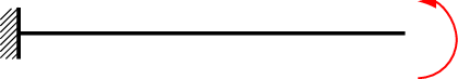
We consider a beam which is fixed at the left boundary and we will apply a moment at the right boundary such that the beam should roll up to a circle (Possion ratio $\bar{ν} = 0$ ). We use loadsteps to increase the moments and apply Newton’s method. As the bending moment would be incorporated strongly via $σ_{\hat{μ} \hat{μ}}$ , which is tedious, we use the hybridized formulation such that we can include the force weakly directly in the formulation.

thickness = 0.1
L = 12
W = 1
E, nu = 1.2e6, 0
moment = IfPos(x - L + 1e-6, 1, 0) * 50 * pi / 3

mapping = lambda x, y, z: (L * x, W * y, 0)
rect = Rectangle(L, W).Face()
rect.edges.Min(X).name = "left"
rect.edges.Max(X).name = "right"
rect.edges.Min(Y).name = "bottom"
rect.edges.Max(Y).name = "top"
mesh = Mesh(OCCGeometry(rect).GenerateMesh(maxh=1))
Draw(mesh);

Due to hybridization the essential and natural boundary conditions swapped again. For the Lagrange multiplier, which has the physical meaning of the rotated angle, we set homogeneous Dirichlet at the clamped left boundary.

order = 2

fes1 = HDivDivSurface(mesh, order=order - 1, discontinuous=True)
fes2 = VectorH1(
    mesh,
    order=order,
    dirichletx_bbnd="left",
    dirichlety_bbnd="left|bottom|top",
    dirichletz_bbnd="left",
)
fes3 = NormalFacetSurface(mesh, order=order - 1, dirichlet_bbnd="left|bottom|top")
fes = fes2 * fes1 * fes3
u, sigma, hyb = fes.TrialFunction()
sigma, hyb = sigma.Trace(), hyb.Trace()

fesRegge = HCurlCurl(mesh, order=order - 1)

gf_solution = GridFunction(fes, name="solution")

Define again the tensors and deformed vectors

Ptau = Id(mesh.dim) - OuterProduct(nv, nv)
Ftau = Grad(u).Trace() + Ptau
Etautau = 0.5 * (Ftau.trans * Ftau - Ptau)

nv_def = Normalize(Cof(Ftau) * nv)
tv_def = Normalize(Ftau * tv)
cnv_def = Cross(nv_def, tv_def)

H_nv_def = (u.Operator("hesseboundary").trans * nv_def).Reshape((3, 3))

Stuff for averaging normal vector and material laws

gf_clamped_bnd = GridFunction(FacetSurface(mesh, order=0))
gf_clamped_bnd.Set(1, definedon=mesh.BBoundaries("left"))

cf_nv_cur = Normalize(Cof(Ptau + Grad(gf_solution.components[0])) * nv)

fesVF = VectorFacetSurface(mesh, order=order)
averaged_nv = GridFunction(fesVF)
averaged_nv_init = GridFunction(fesVF)

averaged_nv.Set(nv, dual=True, definedon=mesh.Boundaries(".*"))
averaged_nv_init.Set(nv, dual=True, definedon=mesh.Boundaries(".*"))
cf_averaged_nv_init_norm = Normalize(averaged_nv_init)
cf_proj_averaged_nv = Normalize(averaged_nv - (tv_def * averaged_nv) * tv_def)

Define hybridized energy and set condense=True to condense out bending moment unknown.

bfA = BilinearForm(fes, symmetric=True, condense=True)
# membrane energy
bfA += Variation(
    0.5 * thickness * MaterialNorm(Interpolate(Etautau, fesRegge), E, nu) * ds
)
# bending energy
bfA += Variation(
    (
        -6 / thickness**3 * MaterialNormInv(sigma, E, nu)
        + InnerProduct(H_nv_def + (1 - nv * nv_def) * Grad(nv), sigma)
    )
    * ds
).Compile()
bfA += Variation(
    (
        acos(cnv_def * cf_proj_averaged_nv)
        - acos(cnv * cf_averaged_nv_init_norm)
        + hyb * cnv
    )
    * sigma[cnv, cnv]
    * ds(element_boundary=True)
).Compile()

par = Parameter(0.0)
bfA += Variation(-par * moment * (hyb * cnv) * ds(element_boundary=True))

gf_solution.vec[:] = 0
gf_history = GridFunction(fes, multidim=0)
gf_u, gf_sigma, _ = gf_solution.components
scene_u = Draw(
    gf_u,
    mesh,
    "displacement",
    deformation=gf_u,
    euler_angles=[-20, 0, 0],
);

Average new normal vector and solve with Newton.

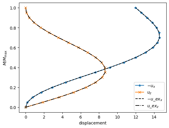
point_P = (L, W / 2, 0)
result_P = [(0, 0, 0)]
ex_sol = [(0, 0, 0)]


def GetExactSolution(par):
    R = 100 / (par.Get() * 50 * pi / 3)
    return (R * sin(L / R) - L, 0, -R * cos(L / R) + R)


tw = widgets.Text(value="step = 0")
display(tw)

num_steps = 20

with TaskManager():
    for steps in range(num_steps):
        par.Set((steps + 1) / num_steps)

        averaged_nv.Set(
            (1 - gf_clamped_bnd) * cf_nv_cur + gf_clamped_bnd * nv,
            dual=True,
            definedon=mesh.Boundaries(".*"),
        )

        solvers.Newton(
            bfA,
            gf_solution,
            inverse="sparsecholesky",
            printing=False,
            maxerr=1e-5,
        )
        scene_u.Redraw()

        result_P.append((gf_u(mesh(*point_P, BND))))
        ex_sol.append(GetExactSolution(par))
        gf_history.AddMultiDimComponent(gf_solution.vec)
        tw.value = f"step = {steps+1}/{num_steps}"

Draw(
    gf_history.components[0],
    mesh,
    animate=True,
    min=0,
    max=12,
    autoscale=True,
    deformation=True,
    euler_angles=[-20, 0, 0],
);

import matplotlib.pyplot as plt

u_x, _, u_z = zip(*result_P)
y_axis = [i / num_steps for i in range(len(u_x))]
u_x = [-val for val in u_x]
u_ex_x, _, u_ex_z = zip(*ex_sol)
u_ex_x = [-val for val in u_ex_x]

plt.plot(u_x, y_axis, "-*", label="$-u_x$")
plt.plot(u_z, y_axis, "-x", label="$u_z$")
plt.plot(u_ex_x, y_axis, "--", color="k", label="$-u\\_ex_x$")
plt.plot(u_ex_z, y_axis, "-.", color="k", label="$u\\_ex_z$")

plt.xlabel("displacement")
plt.ylabel("$M/M_{\\max}$")
plt.legend()
plt.show()

../_images/15a43cf032afdc3e49255ae8bd2fe253e546b6ca9d6e95c8e51e11f16cc8705f.png

We can try out how many rounds the shell can do by further increasing the bending moment.

scene_u = Draw(gf_u, mesh, "displacement", deformation=gf_u)
display(tw)

num_steps = 10
with TaskManager():
    for steps in range(num_steps):
        par.Set(par.Get() + (1) / num_steps)

        averaged_nv.Set(
            (1 - gf_clamped_bnd) * cf_nv_cur + gf_clamped_bnd * nv,
            dual=True,
            definedon=mesh.Boundaries(".*"),
        )
        solvers.Newton(
            bfA,
            gf_solution,
            inverse="sparsecholesky",
            printing=False,
            maxerr=1e-5,
        )
        scene_u.Redraw()
        tw.value = f"step = {steps+1}/{num_steps}"

9.3.2. Nonlinear Naghdi shells with TDNNS#

9.3.2.1. Discretization method#

The Lagrangian for the nonlinear extension of the TDNNS method for Naghdi shells reads [Neunteufel, Schöberl. The Hellan-Herrmann-Johnson and TDNNS method for linear and nonlinear shells. arXiv, (2023).]

\begin{aligned} L (u, σ, γ) & = \int_{S} (\frac{t}{2} ‖ E_{S} (u) ‖_{M}^{2} - \frac{6}{t^{3}} ‖ σ ‖_{C^{- 1}}^{2} + \frac{t κ G}{2} ‖ γ ‖^{2}) d s + \sum_{T \in T} \int_{T} (H_{\tilde{ν}} + (1 - \hat{ν} \cdot \tilde{ν}) \nabla_{S} \hat{ν} - \nabla_{S} γ) : σ d s \\ + \sum_{E \in E} \int_{E} (∢ (ν_{L}, ν_{R}) \circ ϕ - ∢ ({\hat{ν}}_{L}, {\hat{ν}}_{R}) - [[γ_{\hat{μ}}]]) σ_{\hat{μ} \hat{μ}} d l, \end{aligned}

as we consider a hierarchical approach adding additional shearing degrees of freedom on the top of the HHJ method for nonlinear Koiter shells. Here, the director is $\tilde{ν} = ν + F_{S}^{†} γ$ , with $F_{S}^{†}$ the Moore-Penrose pseudo inverse of $F_{S}$ .

9.3.2.2. T-structure#

thickness = 0.1
L = 1
E, nu = 6.2e6, 0
G = E / (2 * (1 + nu))
kappa = 5 / 6

shear = 3e3 * CF((1, 0, 1))

f1 = WorkPlane(Axes((0, 0, 0), n=X, h=Y)).Rectangle(L, L).Face()
f1.edges.Min(Z).name = "bottom"
f1.edges.Max(Z).name = "top"
f1.edges.Min(Y).name = "left"
f1.edges.Max(Y).name = "right"
f2 = WorkPlane(Axes((-L / 2, 0, L), n=Z, h=X)).Rectangle(L, L).Face()
f2.edges.Min(Y).name = "zpbottom"
f2.edges.Max(Y).name = "uptop"
f2.edges.Min(X).name = "upleft"
f2.edges.Max(X).name = "upright"
shape = Glue([f1, f2])
mesh = Mesh(OCCGeometry(shape).GenerateMesh(maxh=0.25))
Draw(mesh, euler_angles=[-60, 0, -15]);

order = 3

fesU = VectorH1(mesh, order=order, dirichlet_bbnd="bottom")
fesM = HDivDivSurface(mesh, order=order - 1, discontinuous=True)
fesH = NormalFacetSurface(mesh, order=order - 1, dirichlet_bbnd="bottom")
fesB = HCurl(mesh, order=order - 1, dirichlet_bbnd="bottom")
fes = fesU * fesM * fesB * fesH

u, sigma, gamma, hyb = fes.TrialFunction()
sigma, gamma, hyb = sigma.Trace(), gamma.Trace(), hyb.Trace()

fesRegge = HCurlCurl(mesh, order=order - 1, discontinuous=True)

gf_solution = GridFunction(fes, name="solution")

Ptau = Id(mesh.dim) - OuterProduct(nv, nv)
Ftau = Grad(u).Trace() + Ptau
Etautau = 0.5 * (Ftau.trans * Ftau - Ptau)


def PseudoInverse(mat, v):
    """Pseudo Inverse of a rank (n-1) matrix
    v needs to lie in the kernel of mat
    """
    return Inv(mat.trans * mat + OuterProduct(v, v)) * mat.trans


nv_def = Normalize(Cof(Ftau) * nv)
tv_def = Normalize(Ftau * tv)
cnv_def = Cross(nv_def, tv_def)
director = nv_def + PseudoInverse(Ftau, nv).trans * gamma

H_nv_def = (u.Operator("hesseboundary").trans * director).Reshape((3, 3))

gf_clamped_bnd = GridFunction(FacetSurface(mesh, order=0))
gf_clamped_bnd.Set(1, definedon=mesh.BBoundaries("left"))

cf_nv_cur = Normalize(Cof(Ptau + Grad(gf_solution.components[0])) * nv)

fesVF = VectorFacetSurface(mesh, order=order)
averaged_nv = GridFunction(fesVF)
averaged_nv_init = GridFunction(fesVF)

averaged_nv.Set(nv, dual=True, definedon=mesh.Boundaries(".*"))
averaged_nv_init.Set(nv, dual=True, definedon=mesh.Boundaries(".*"))
cf_averaged_nv_init_norm = Normalize(averaged_nv_init)
cf_proj_averaged_nv = Normalize(averaged_nv - (tv_def * averaged_nv) * tv_def)

Define the bilinear form for the problem including membrane, bending, and shearing energy.

bfA = BilinearForm(fes, symmetric=True, condense=True)
# Membrane energy
bfA += Variation(
    0.5 * thickness * MaterialNorm(Interpolate(Etautau, fesRegge), E, nu) * ds
).Compile()
# Bending energy
bfA += Variation(
    (
        -6 / thickness**3 * MaterialNormInv(sigma, E, nu)
        + InnerProduct(H_nv_def + (1 - nv * director) * Grad(nv) - Grad(gamma), sigma)
    )
    * ds
).Compile()
bfA += Variation(
    (
        acos(cnv_def * cf_proj_averaged_nv)
        - acos(cnv * cf_averaged_nv_init_norm)
        + hyb * cnv
        + (PseudoInverse(Ftau, nv).trans * gamma) * cnv_def
    )
    * sigma[cnv, cnv]
    * ds(element_boundary=True)
).Compile()
# Shear energy
bfA += Variation(0.5 * thickness * kappa * G * gamma * gamma * ds)

par = Parameter(0.0)
bfA += Variation(-par * shear * u * dx(definedon=mesh.BBoundaries("upleft")))

gf_solution.vec[:] = 0
gf_history = GridFunction(fes, multidim=0)

gfu, gfsigma, gfgamma, _ = gf_solution.components

scene = Draw(gfu, mesh, "displacement", deformation=gfu, euler_angles=[-60, 0, -10])
scene2 = Draw(
    Norm(gfsigma),
    mesh,
    "bending_stress",
    deformation=gfu,
    euler_angles=[-60, 0, -10],
)
scene3 = Draw(
    thickness * kappa * G * gfgamma,
    mesh,
    "shear_stress",
    deformation=gfu,
    euler_angles=[-60, 0, -10],
)

num_steps = 20

tw = widgets.Text(value="step = 0")
display(tw)

with TaskManager():
    for steps in range(num_steps):
        par.Set((steps + 1) / num_steps)

        averaged_nv.Set(
            (1 - gf_clamped_bnd) * cf_nv_cur + gf_clamped_bnd * nv,
            dual=True,
            definedon=mesh.Boundaries(".*"),
        )

        solvers.Newton(
            bfA,
            gf_solution,
            inverse="sparsecholesky",
            printing=False,
            maxerr=1e-5,
        )
        scene.Redraw()
        scene2.Redraw()
        scene3.Redraw()

        gf_history.AddMultiDimComponent(gf_solution.vec)
        tw.value = f"step = {steps+1}/{num_steps}"

Draw(
    gf_history.components[0],
    mesh,
    animate=True,
    min=0,
    max=1.25,
    autoscale=True,
    deformation=True,
    euler_angles=[-60, 0, -10],
);