16. 3D Skeleton Block Jacobi Preconditioner

A preconditioner for the Helmholtz equation

\[\begin{alignat*}{2} -\Delta u - \kappa^2 u &= 0 \quad && \text{ in } \Omega, \\ \nabla u \cdot \mathbf{n} + j \kappa u &= g \quad && \text{ on } \partial \Omega \end{alignat*}\]

is introduced. It is based upon the mixed hybrid Discontinous Galerkin (HDG) formulation introduced in Hybridizing Raviart-Thomas Elements for the Helmholtz Equation. For the HDG formulation static condensation is emploid and for the resulting system of linear equations on the skeleton, a block Jacobi Preconditioner is applied. For more information about the formulation in combination with iterative solver strategies see Hybrid discontinuous Galerkin methods for the wave equation.

16.1. Geometry

The following simple cube with spheres as scattereres inside and a Gauß-peak on the left as excitation is considered as an example.

from netgen.occ import *
from ngsolve import *
from ngsolve.webgui import Draw
clipping = { "clipping" : {"z":-1, "dist":0, "function":True} }

maxh = 0.15 #0.1
l = 2 #number spheres in y-direction
m = 1 #number spheres in z-direction
cube = Box( (-1,-1,-1), (1,1,1)).bc("transparent")
cube.faces[0].name = "excitation"

#add spheres
dist = 0.3
radius = dist/3
yoff = -dist*(l-1)/2
zoff = -dist*(m-1)/2
for it in range(l):
    for jt in range(m):
        cube = cube - Sphere(Pnt(0, yoff + dist*it, zoff + dist*jt), radius).bc("dirichlet")
        
visplane = HalfSpace(Pnt(0,0,0), Vec(0,0,1))
backC = cube*visplane
frontC = cube-visplane
geo = OCCGeometry([backC, frontC])
mesh = geo.GenerateMesh(maxh = maxh)
mesh = Mesh(mesh)
mesh.Curve(3)
Draw(mesh, **clipping, draw_vol=False, draw_surf=True, order=1);

p = 2 #fem order
k = 30 # #wavenumber

lam = 2*pi/k
print("wavelength:", lam)
print("number waves in domain:", 2/lam)
transbnd = "transparent|excitation"
excbnd = "excitation"
scattererbnd = "dirichlet"
excitation = -1e1*k*1j*exp(-2e1*(y**2 + z**2))

wavelength: 0.20943951023931953
number waves in domain: 9.549296585513721

16.2. Weak HDG Formulation

The mixed formulation is stated on the space \(L_2(\Omega) \times H_{pw}(div, \Omega) \times L_2(\mathcal{F}) \times L_2(\mathcal{F})\) with the sesquilinearform

\[\begin{alignat*}{2} s(u, \sigma, \hat u, \hat \sigma; v, \tau, \hat v, \hat \tau) := \sum_{T \in \mathcal{T}}\int_T j\kappa u v - div(\sigma) v - u div(\tau) - j \kappa \sigma \tau d\mathbf{x} + \int_{\partial T} \sigma \cdot \mathbf{n} \hat v + \hat u \tau \cdot \mathbf{n} d \mathbf{s} \\ + \int_{\partial T} 2(\sigma - \hat \sigma) \cdot \mathbf{n} (\tau - \hat \tau) \cdot \mathbf{n} - \frac{1}{2}(\Pi^p u - \hat u) (\Pi^p v - \hat v) d\mathbf{s} - \int_{\partial \Omega} \hat u \hat v d \mathbf{s}. \end{alignat*}\]

In the sesquilinearform condensation is enabled and internal elements matrices are not stored to reduce the memory consumption. This implies that at the end the solution need to be extended from skeleton unknowns onto elements. The method of projected jumps by Schöberl and Lehrenfeld is applied to increase the polynomial order of the scalar variable \(u\) on elements.

U = L2(mesh, order=p+1, complex=True)
V = Discontinuous(HDiv(mesh, order=p, complex=True, RT=True)) # P^k Sub RT Sub P^k+1, div(RT) = P^k
FD = FacetFESpace(mesh, order=p+1, complex=True, highest_order_dc = True, dirichlet = scattererbnd)
FN = NormalFacetFESpace(mesh, order=p, complex=True)
X = U*V*FD*FN
print("nDof:", X.ndof, "(u", U.ndof, ", sigma", V.ndof, ", uhat", FD.ndof, ", sigmahat", FN.ndof, ")")

nDof:

 1622412 (u 334780 , sigma 602604 , uhat 476426 , sigmahat 208602 )

(u, sigma, uhat, sigmahat), (v, tau, vhat, tauhat) = X.TnT()
n = specialcf.normal(mesh.dim)
dS = dx(element_boundary=True)

a = BilinearForm(X, condense = True, eliminate_internal=True)

a += (1j*k*u*v - div(sigma)*v - u*div(tau) - 1j*k*sigma*tau) *dx
a += (sigma*n*vhat + uhat*tau*n) *dS
a += (2*(sigma-sigmahat)*n*(tau-tauhat)*n -1/2*(u-uhat)*(v-vhat)) *dS
a += -uhat.Trace()*vhat.Trace() *ds(definedon=mesh.Boundaries(transbnd))

f = LinearForm(X)
f += -1/k**2 * excitation * vhat.Trace() *ds(definedon = mesh.Boundaries(excbnd))

16.3. Skeleton Block Jacobi Preconditioner in 3D

The unknowns on a face are combined into a block for the block Jacobi preconditioner.

def GenerateBlocks3D(ablf, mesh, X, GS=False):
    freedofs = X.FreeDofs()
    print("Collect smoothing blocks")
    blocks = []
    for facet in mesh.facets:
        vdofs = []
        facedofs = X.GetDofNrs(facet)
        for fdof in facedofs:
            if freedofs[fdof]:
                vdofs.append(fdof)
        #blocks.append (tuple(X.GetDofNrs(facet)))
        blocks.append(vdofs)
    print("Create block smoother")
    blockjacobi = ablf.mat.CreateBlockSmoother(blocks, GS=GS)
    return blockjacobi

gfu = GridFunction(X)
with TaskManager():
    print("Assemble a")
    a.Assemble()
    print("Assemble f")
    f.Assemble()
    blockinvs = GenerateBlocks3D(a, mesh, X, GS=False)
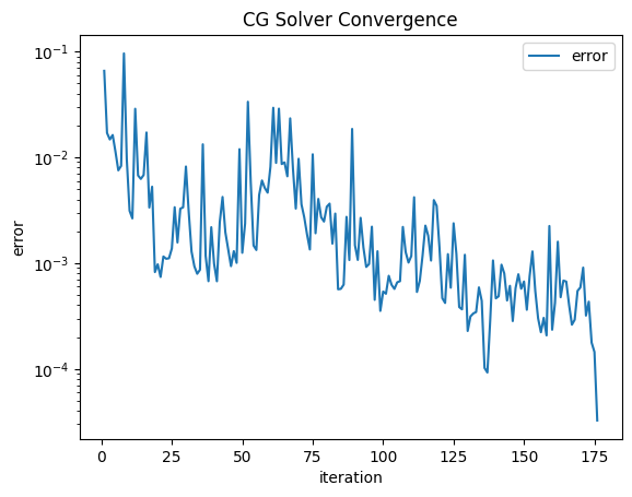
    solvers.CG(mat=a.mat, rhs=f.vec, sol=gfu.vec, pre=blockinvs, maxsteps=1000, tol=1e-3, plotrates=True)
    print("Compute internal solution")
    a.ComputeInternal (gfu.vec, f.vec)
    print("Done")

Compute internal solution

Done

<Figure size 640x480 with 0 Axes>

Draw(BoundaryFromVolumeCF(gfu.components[0]), mesh, "press", min=-0.03, max=0.03, \
     draw_surf=True, draw_vol=False, order=3, animate_complex=True, **clipping);