8.1.1. Reissner-Mindlin plate#

Assuming a thin three-dimensional plate $\mathrm{\Omega }=(0,1{)}^2\times (-t/2,t/2)$ we can perform a dimension reduction to the mid-surface $\mathcal{S}=(0,1{)}^2\times \{0\}$. We assume the structure to be clamped on all boundaries except the top and bottom one, where homogeneous Neumann boundary conditions are prescribed. We postulate kinematic assumptions, which are named after Reissner and Mindlin:

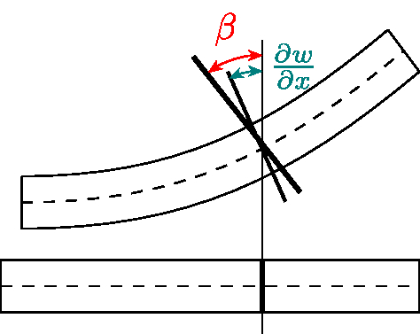
1. Lines normal to the mid-surface get deformed linearly, they remain lines.

2. The displacements in $z$-direction are independent of the $z$-coordinate.

3. Points on the mid-surface can only be deformed in $z$-direction.

4. Stresses ${\sigma }_{33}$ in normal direction vanish (called plane-stress assumption).

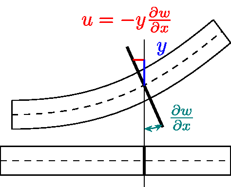
With H1-H3 the displacements are of the form

Hypothesis H3 directly enforces that the horizontal displacements of the membrane problem is eliminated and yields together with H1 the form of the shearing related horizontal displacements $u_1$ and $u_2$. H2 in combination with H1 gives the form of the vertical displacement. Assumption H4 is needed as from $u_3=w(x,y)$ there follows ${\epsilon }_{33}(u)=0$, i.e., no strains in thickness direction. Using the stress-strain relation to compute ${\sigma }_{33}$ yields ${\sigma }_{33}=\frac{E}{(1+\nu )(1-2\nu )}((1-\nu ){\epsilon }_{33}+\nu ({\epsilon }_{11}+{\epsilon }_{22}))=\lambda ({\epsilon }_{11}+{\epsilon }_{22})\ne 0$ in general. This is non-physical and leads to a not asymptotically correct model. It induces a too stiff behavior yielding artificial stiffness. Therefore ${\sigma }_{33}=0$ is postulated to re-obtain an asymptotically correct model, which converges to the 3D solution in the limit of vanishing thickness. Setting ${\sigma }_{33}=0$ induces that the material can stretch in thickness direction without inducing stresses.

The 3D elasticity strain tensor reads

From H4, ${\sigma }_{33}=0$, we can express ${\epsilon }_{33}=-\frac{\nu }{1-\nu }({\epsilon }_{11}+{\epsilon }_{22})$ by using the stress-strain relation $\sigma =\mathbb{C}\epsilon$

and reinserting yields

For example, there holds

The energy $\Vert \epsilon {\Vert }_{\mathbb{C}}^2=\mathbb{C}\epsilon :\epsilon =\sigma :\epsilon$ reads

Next, we integrate the arising terms over the thickness and insert the strain definition

where $\underset{―}{\mathrm{\nabla }}$, $\underset{―}{\epsilon }$, and $\underset{―}{\mathrm{div}}$ denote the differential operators acting only on the first two indices $i,j=1,2$.

Thus, the total energy $W(w,\beta )=\frac{1}{2}{\int }_{\mathrm{\Omega }}\sigma :\epsilon d(x,y,z)$ becomes with the notation $ds=d(x,y)$

where $G=\frac{E}{2(1+\nu )}$ denotes the shearing modulus. Classically, the shear correction factor $\kappa =\frac{5}{6}$ is additionally inserted into the shearing energy term to compensate high-order effects of the shear stresses, which are not constant through the thickness (in some variational methods to derive plate equations the factor $5/6$ directly appears).

The right-hand side $f$ is assumed to act only vertically on the plate and is independent of the thickness $f=(0,0,f^z(x,y))$. Integrating over the thickness and rescaling $f:=t^{-2}{f}^z$ leads to the term $t^3{\int }_{\mathcal{S}}fvds$.

To simplify notation we set $\mathrm{\Omega }=\mathcal{S}$, use $dx$ for integration over the mid-surface, neglect the underline for the differential operators, and define the plate elasticity tensor

All together, taking the variations of the Reissner-Mindlin plate energy (with the shear correction factor $\kappa$) and dividing by $t^3$ yields the clamped Reissner-Mindlin plate equation: Find $(w,\beta )\in H_0^1(\mathrm{\Omega })\times [H_0^1(\mathrm{\Omega }){]}^2$ such that for all $(v,\delta )\in H_0^1(\mathrm{\Omega })\times [H_0^1(\mathrm{\Omega }){]}^2$

Depending on the different combination of Dirichlet (D) and Neumann (N) boundary conditions for the vertical deflection $w$ and the rotations $\beta$ we distinguish between the following plate boundary conditions. Let $M:=\frac{1}{12}\mathbb{D}\epsilon (\beta )$ be the bending moment tensor and $Q:=\frac{\kappa G}{t^2}(\mathrm{\nabla }w-\beta )$ the shear force.

8.1.2. Kirchhoff-Love plate#

For thin plates like metal sheets the Kirchhoff-Love hypothesis is assumed additionally to H1-H4.

5. Lines normal to the mid-surface are after deformation again normal to the deformed mid-surface.

It states that normal vectors of the original plate stay perpendicular to the mid-surface of the deformed plate. This means that no shearing occurs, i.e., the rotations $\beta$ from the Reissner-Mindlin plate equation can be eliminated by the gradient of the vertical deflection $w$ of the mid-surface, $\beta =\mathrm{\nabla }w$. Note, that $\mathrm{\nabla }w$ is the linearization of the rotated normal vector of the plate.

Eliminating $\beta$ from the Reissner-Mindlin plate equation leads to the Kirchhoff-Love plate equation, which is a fourth order problem. Assuming clamped boundary conditions it reads: Find $w\in H_0^2(\mathrm{\Omega })$ such that for all $v\in H_0^2(\mathrm{\Omega })$

The thickness parameter $t$ does not enter the equation. The problem is well-posed for $w\in H_0^2(\mathrm{\Omega })$ and reads in strong form

Additionally to clamped boundary conditions also free and simply supported boundary conditions can be prescribed. The general case in strong form reads:

where the boundary $\mathrm{\Gamma }=\partial \mathrm{\Omega }$ splits into clamped, simply supported, and free boundaries ${\mathrm{\Gamma }}_c$, ${\mathrm{\Gamma }}_s$, and ${\mathrm{\Gamma }}_f$, respectively. ${\mathcal{V}}_{{\mathrm{\Gamma }}_f}$ denotes the set of corner points where the two adjacent edges belong to ${\mathrm{\Gamma }}_f$. Here, $n$ and $t$ denote the outer normal and tangential vector on the plate boundary. Physically, ${\sigma }_{nn}:=n^{\mathrm{\top }}\sigma n$ is the normal bending moment, ${\partial }_t(t^{\mathrm{\top }}\sigma n)+n^{\mathrm{\top }}\mathrm{div}(\sigma )$ the effective transverse shear force, and ${\sigma }_{nt}:=t^{\mathrm{\top }}\sigma n$ the torsion moment. Further, the shear force $Q$ is given by $Q=-\mathrm{div}(\sigma )$.