7. Elastodynamics with Newmark and generalized-alpha time-stepping

\(u\) … displacement, \(v = \dot u \) … velocity, \(a = \dot v\) .. acceleration

Newmark scheme, see tutorial Newmark:

\[\begin{align*} \frac{u^{n+1}-u^n}{\tau} = \frac{v^n+v^{n+1}}{2} \\ \frac{v^{n+1}-v^n}{\tau} = \frac{a^n+a^{n+1}}{2} \\ \end{align*}\]

with new acceleration, with elasticity operator \(K\):

\[\begin{align*} a^{n+1} = f - K(u^{n+1}) \end{align*}\]

By inserting the definition of \(a^{n+1}\) and \(v^{n+1}\) we obtain a nonlinear problem in \(u^{n+1}\). Then, we can update the velocity and acceleration.

from ngsolve import *
from ngsolve.webgui import Draw
import ipywidgets as widgets
from netgen.occ import *

shape = Rectangle(1, 0.1).Face()
shape.edges.Max(X).name = "right"
shape.edges.Min(X).name = "left"
shape.edges.Max(Y).name = "top"
shape.edges.Min(Y).name = "bot"
shape.vertices.Min(X + Y).maxh = 0.01
shape.vertices.Min(X - Y).maxh = 0.01
mesh = Mesh(OCCGeometry(shape, dim=2).GenerateMesh(maxh=0.05))
Draw(mesh);

E, nu = 210, 0.2
mu = E / 2 / (1 + nu)
lam = E * nu / ((1 + nu) * (1 - 2 * nu))


def NeoHooke(C):
    return 0.5 * mu * (Trace(C - Id(2)) + 2 * mu / lam * Det(C) ** (-lam / 2 / mu) - 1)


tau = 0.02
tend = 20
force = CF((0, -1))

fes = VectorH1(mesh, order=3, dirichlet="left")
u, v = fes.TnT()
C = (Id(2) + Grad(u)).trans * (Id(2) + Grad(u))

gfu = GridFunction(fes)
gfv = GridFunction(fes)
gfa = GridFunction(fes)
gfuold = GridFunction(fes)
gfvold = GridFunction(fes)
gfaold = GridFunction(fes)

bfa = BilinearForm(fes)
bfa += Variation(NeoHooke(C) * dx)

vel_new = 2 / tau * (u - gfuold) - gfvold
acc_new = 2 / tau * (vel_new - gfvold) - gfaold

bfa += acc_new * v * dx
bfa += -force * v * dx

gfu_history = GridFunction(fes, multidim=0)
sceneu = Draw(
    gfu,
    deformation=True,
    settings={
        "camera": {"transformations": [{"type": "move", "dir": (0, 0, 1), "dist": -2}]}
    },
)
scenev = Draw(gfv)
gfu.vec[:] = 0
t = 0
step = 0

tw = widgets.Text(value="t = 0")
display(tw)

while t < tend:
    t += tau
    step += 1
    solvers.Newton(a=bfa, u=gfu, printing=False, inverse="sparsecholesky")

    gfv.vec[:] = 2 / tau * (gfu.vec - gfuold.vec) - gfvold.vec
    gfa.vec[:] = 2 / tau * (gfv.vec - gfvold.vec) - gfaold.vec

    sceneu.Redraw()
    scenev.Redraw()

    gfuold.vec[:] = gfu.vec
    gfvold.vec[:] = gfv.vec
    gfaold.vec[:] = gfa.vec
    if step % 30 == 0:
        gfu_history.AddMultiDimComponent(gfu.vec)
    tw.value = f"t = {t}"

Draw(
    gfu_history,
    mesh,
    interpolate_multidim=True,
    animate=True,
    min=0,
    max=1,
    autoscale=False,
    deformation=True,
    settings={
        "camera": {"transformations": [{"type": "move", "dir": (0, 0, 1), "dist": -2}]}
    },
);

7.1. Rotor with Newmark time stepping

We consider a rotor, which is completely free and undergoes at the beginning a skew-symmetric force to start rotating. Then it should infinitely rotate as the force is given away. However, after sufficiently many time-steps the finite element solution starts inducing high frequency modes. These frequencies cannot be resolved sufficiently enough by the finite element solution and the system becomes unstable.

from ngsolve import *
from ngsolve.webgui import Draw
from netgen.occ import *
import ipywidgets as widgets

shape = MoveTo(-5, -0.5).Rectangle(10, 1).Face()
mesh = Mesh(OCCGeometry(shape, dim=2).GenerateMesh(maxh=0.5))

tend = 30
tau = Parameter(0.06)

par = Parameter(0.0)
force = 10 * par * CoefficientFunction((0, x))


def Force(t):
    f = 0.5
    if t < f + tau.Get() / 2:
        return t / f
    return 0


E, nu = 2e3, 0.2
mu = E / 2 / (1 + nu)
lam = E * nu / ((1 + nu) * (1 - 2 * nu))


def NeoHooke(C):
    return (
        0.5 * mu * (Trace(C - Id(2)) + 2 * mu / lam * (Det(C) ** (-lam / 2 / mu) - 1))
    )


fes = VectorH1(mesh, order=3, dirichlet="left")
u, v = fes.TnT()
C = (Id(2) + Grad(u)).trans * (Id(2) + Grad(u))

gfu = GridFunction(fes)
gfv = GridFunction(fes)
gfa = GridFunction(fes)
gfuold = GridFunction(fes)
gfvold = GridFunction(fes)
gfaold = GridFunction(fes)

bfa = BilinearForm(fes)
bfa += Variation(NeoHooke(C) * dx)

vel_new = 2 / tau * (u - gfuold) - gfvold
acc_new = 2 / tau * (vel_new - gfvold) - gfaold

bfa += acc_new * v * dx
bfa += -force * v * dx

gfu_history = GridFunction(fes, multidim=0)
gfv_history = GridFunction(fes, multidim=0)
sceneu = Draw(gfu, deformation=True)
scenev = Draw(gfv)
gfu.vec[:] = 0
t = 0
step = 0

tw = widgets.Text(value="t = 0")
display(tw)

while t < tend:
    par.Set(Force(t))
    step += 1
    result, _ = solvers.Newton(a=bfa, u=gfu, printing=False, inverse="sparsecholesky")
    if result == -1:
        print(f"Newton did not converge at t={t}")
        break

    gfv.vec[:] = 2 / tau.Get() * (gfu.vec - gfuold.vec) - gfvold.vec
    gfa.vec[:] = 2 / tau.Get() * (gfv.vec - gfvold.vec) - gfaold.vec

    sceneu.Redraw()
    scenev.Redraw()

    gfuold.vec[:] = gfu.vec
    gfvold.vec[:] = gfv.vec
    gfaold.vec[:] = gfa.vec
    if step % 10 == 0:
        gfu_history.AddMultiDimComponent(gfu.vec)
        gfv_history.AddMultiDimComponent(gfv.vec)
    t += tau.Get()
    tw.value = f"t = {t}"

Warning: Newton might not converge! Error =  1257.7961064970277
Newton did not converge at t=20.219999999999953

Draw(
    gfv_history,
    mesh,
    interpolate_multidim=True,
    animate=True,
    min=0,
    max=9,
    autoscale=False,
    deformation=gfu_history,
);

7.2. Generalized alpha method

Reference: [Chung, Hulbert. A time Integration Algorithm for Structural Dynamics With Improved Numerical Dissipation: The Generalized-\(\alpha\) Method. J. Appl. Mech. 1993]

Solve at each time step

\[\begin{align*} M\,a_{n+1-\alpha_m}= F(x_{n+1-\alpha_f}), \end{align*}\]

where

\[\begin{align*} x_{n+1} &= x_n + \tau\,v_n + \tau^2\big((\frac{1}{2}-\beta)a_n+\beta\,a_{n+1}\big),\\ v_{n+1}&= v_n + \tau((1-\gamma)a_n+\gamma\,a_{n+1}),\\ x_{n+1-\alpha_f}&= (1-\alpha_f)x_{n+1}+\alpha_fx_n,\\ a_{n+1-\alpha_m}&= (1-\alpha_m)a_{n+1}+\alpha_ma_n. \end{align*}\]

By inserting into definitions we obtain the following scheme: For given \(x_n\), \(v_n\), and \(a_n\) solve the following nonlinear problem in \(a_{n+1}\)

\[\begin{align*} M\,\big((1-\alpha_m)a_{n+1}+\alpha_ma_n\big)= F\Big(x_n+(1-\alpha_f)\Big[\tau\,v_n + \tau^2(\big(\frac{1}{2}-\beta\big)a_n+\beta\,a_{n+1})\Big]\Big). \end{align*}\]

Then compute \(x_{n+1}\) and \(v_{n+1}\) via the first two update formulas above.

The method depends on the free parameter \(\rho^\infty\) from which the other parameters follow as

\[\begin{align*} \alpha_m &= \frac{2\rho^\infty-1}{\rho^\infty+1},\\ \alpha_f &= \frac{\rho^\infty}{\rho^\infty+1},\\ \beta &= \frac{1}{4}(1-\alpha_m+\alpha_f)^2,\\ \gamma &= \frac{1}{2}-\alpha_m+\alpha_f. \end{align*}\]

The parameter \(\rho^\infty\) defines the damping for high frequency functions. Therefore, the ground movement of the structure is preserved and only little energy of the system is lost, even with a strong damping \(\rho^\infty < 1\).

from ngsolve import *
from ngsolve.webgui import Draw
from netgen.occ import *
import ipywidgets as widgets

shape = MoveTo(-5, -0.5).Rectangle(10, 1).Face()
mesh = Mesh(OCCGeometry(shape, dim=2).GenerateMesh(maxh=0.5))

tend = 50
tau = Parameter(0.06)

par = Parameter(0.0)
force = 10 * par * CoefficientFunction((-y, x))


def Force(t):
    f = 0.5
    if t < f + tau.Get() / 2:
        return t / f
    return 0


E, nu = 2e3, 0.2
mu = E / 2 / (1 + nu)
lam = E * nu / ((1 + nu) * (1 - 2 * nu))

# damping parameter. Try out 0.5, 0.8, and 0.95
rho = Parameter(0.8)
print(f"rho = {rho.Get()}")

# generalized alpha parameters
am = (2 * rho.Get() - 1) / (rho.Get() + 1)
af = rho.Get() / (rho.Get() + 1)
beta = 0.25 * (1 - am + af) ** 2
gamma = 0.5 - am + af


order = 2
V = VectorH1(mesh, order=order)
a, at = V.TnT()


def NeoHooke(C):
    return (
        0.5 * mu * (Trace(C - Id(2)) + 2 * mu / lam * (Det(C) ** (-lam / 2 / mu) - 1))
    )


def Stress(C):
    return 0.5 * mu * (Id(2) - Det(C) ** (-lam / 2 / mu) * Inv(C))


gfa = GridFunction(V)
uold = GridFunction(V)
vold = GridFunction(V)
aold = GridFunction(V)


# Grad(x_{n+1-a_f})
grad_x = Grad(uold) + (1 - af) * (
    tau * Grad(vold) + tau * tau * ((0.5 - beta) * Grad(aold) + beta * Grad(a))
)
Fa = grad_x + Id(2)
Ca = Fa.trans * Fa

B = BilinearForm(V, symmetric=False)
B += (a * at * (1 - am) + am * aold * at) * dx
B += (2 * InnerProduct(Stress(Ca), Fa.trans * Grad(at)) - force * at) * dx

gfu_history = GridFunction(V, multidim=0)
gfv_history = GridFunction(V, multidim=0)
scene = Draw(vold, mesh, "velocity", deformation=uold)

# kinematic and potential energy
F = Grad(a) + Id(2)
C = F.trans * F
bf_kinetic_energy = BilinearForm(V, symmetric=True)
bf_kinetic_energy += Variation(0.5 * a * a * dx)
bf_potential_energy = BilinearForm(V, symmetric=True)
bf_potential_energy += Variation(NeoHooke(C) * dx)

rho = 0.8

result = [(0, 0)]

tw = widgets.Text(value="t = 0")
display(tw)

t = 0
step = 0
with TaskManager():
    while t < tend - tau.Get() / 2:
        par.Set(Force(t))
        aold.vec.data = gfa.vec

        converged, _ = solvers.Newton(B, gfa, maxerr=1e-10, printing=False)
        if converged == -1:
            print(f"No convergence at t={t}!")
            break

        # update displacement and velocity
        uold.vec.data += tau.Get() * vold.vec + tau.Get() ** 2 * (
            (0.5 - beta) * aold.vec + beta * gfa.vec
        )
        vold.vec.data += tau.Get() * ((1 - gamma) * aold.vec + gamma * gfa.vec)

        scene.Redraw()

        if step % 10 == 0 and t < 30:
            gfu_history.AddMultiDimComponent(uold.vec)
            gfv_history.AddMultiDimComponent(vold.vec)

        t += tau.Get()
        result.append(
            (
                t,
                bf_kinetic_energy.Energy(vold.vec)
                + bf_potential_energy.Energy(uold.vec),
            )
        )
        tw.value = f"t = {t}"
        step += 1

Draw(
    gfv_history,
    mesh,
    interpolate_multidim=True,
    animate=True,
    min=0,
    max=9,
    autoscale=False,
    deformation=gfu_history,
);

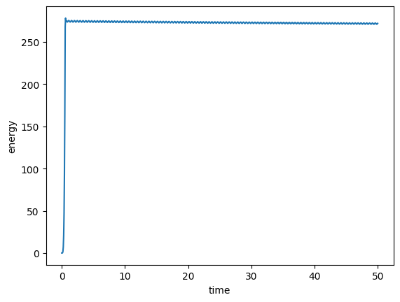
Plot total energy \(E=E_{\mathrm{kin}}+E_{\mathrm{pot}}\) over time. For \(\rho^\infty=0.8\) we see a stable oscillation around a constant energy level. A strong damping of \(\rho^\infty=0.5\) leads to an increase of the total energy of the system. The reduction, however, becomes less over time and the rotation movement remains. The internal elastic oscillation are damped such that the global rigid body rotation remains. (\(\rho^\infty=0.95\) becomes unstable.)

import matplotlib.pyplot as plt

t, energy = zip(*result)
plt.xlabel("time")
plt.ylabel("energy")
plt.plot(t, energy, "-")
plt.show()