Normal-cont. HDG tricks

11.5. Normal-cont. HDG tricks#

We now turn over to the \(H(\operatorname{div})\)-HDG Stokes discretization:

We will first a discuss how to apply the facet dof reduction
Afterwards, we will explain a relaxed \(H(\operatorname{div})\)-conforming discretizations to obtain a reduction of facet dofs also for the normal-continuity dofs
Finally, we will exploit knowledge about the pointwise divergence of the discrete solution (it’s zero) to reduce the local FESpaces

11.5.1. Projected jumps for the `TangentialFacetFESpace`#

For the \(H(\operatorname{div})\)-HDG Stokes discretization we can apply the “projected jumps” modification as well, simply adding the same frags and the compression on the TangentialFacetFESpace. We will apply it below, after introducing further tuning tricks.

Note

Making the highest order dofs discontinuous is implemented for the facet spaces FacetFESpace, TangentialFacetFESpace and NormalFacetFESpace through the highest_order_dc flag. Further, the flag hide_highest_order_dc is implemented for all these spaces.

11.5.2. Relaxed \(H(\operatorname{div})\)-conforming `FESpace`s#

After reducing the globally coupled tangential facet dofs we have degrees of freedom of order \(k-1\) on the facets for the tangential component, but still order \(k\) for the normal component (as we are in \(H(\operatorname{div})\). In view of an optimal dof-reduction on the facets we can do even better:

By relaxing \(H(\operatorname{div})\)-conformity. Here, we again take the dofs for the highest order normal component and only for that we break up continuity, turning (again) one INTERFACE_DOF into two LOCAL_DOFs:

→

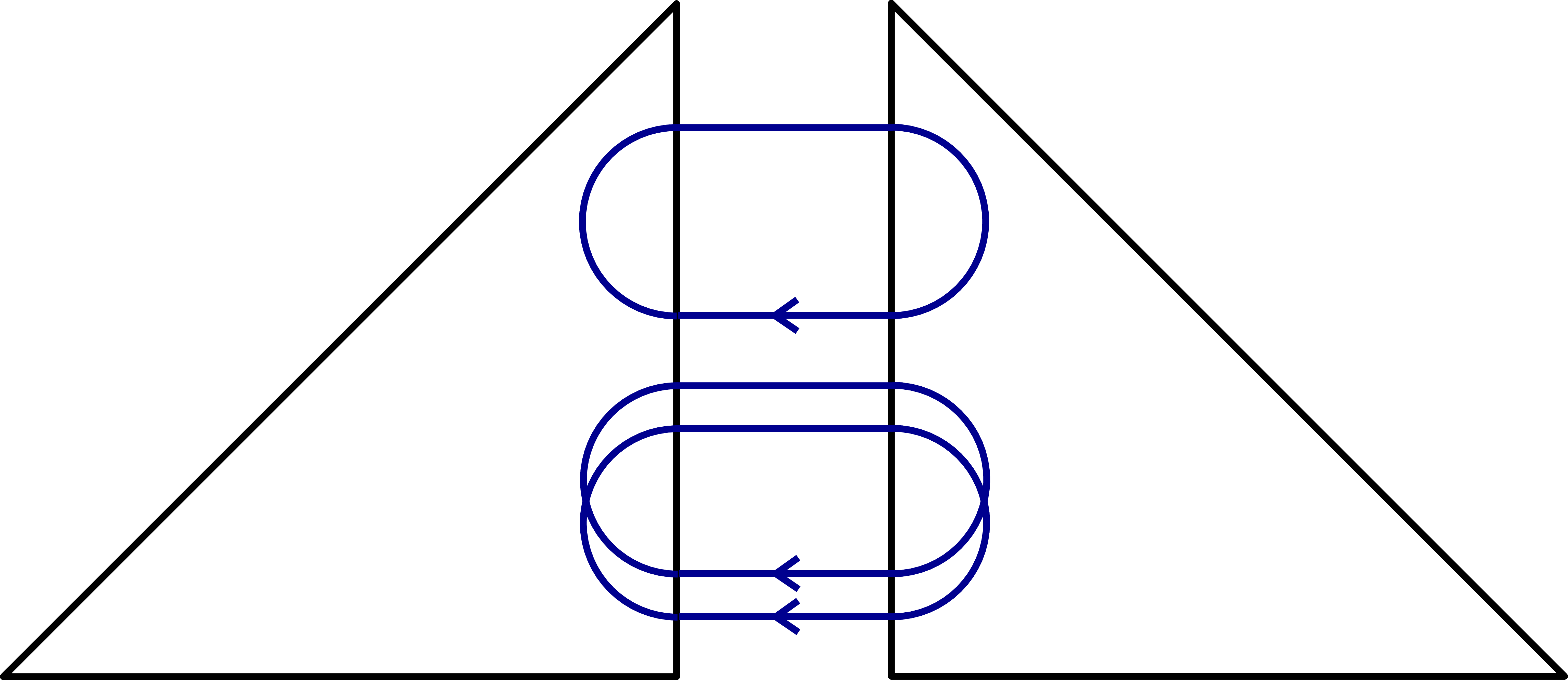The resulting velocity space (without the facet space) is

\[ V_h^T = \{ v \in [\mathbb{P}^k]^d(\mathcal{T}_h) \mid [\![\Pi^{k-1}_{\mathcal{T}_h} v \cdot n ]\!] = 0 \text{ on } \mathcal{F}_h\} \]

where \([\![\cdot]\!]\) is the usual DG jump operator.

The relaxed \(H(\operatorname{div})\)-version of the HDiv-space in NGSolve is obtained with the highest_order_dc flag:

HDiv(mesh, ..., highest_order_dc=True)

Note

Breaking up the highest order continuity using the flag highest_order_dc is implemented in NGSolve also for the FESpaces: TangentialFacetFESpace, NormalFacetFESpace, HDiv, HCurl, H1, HDivSurface

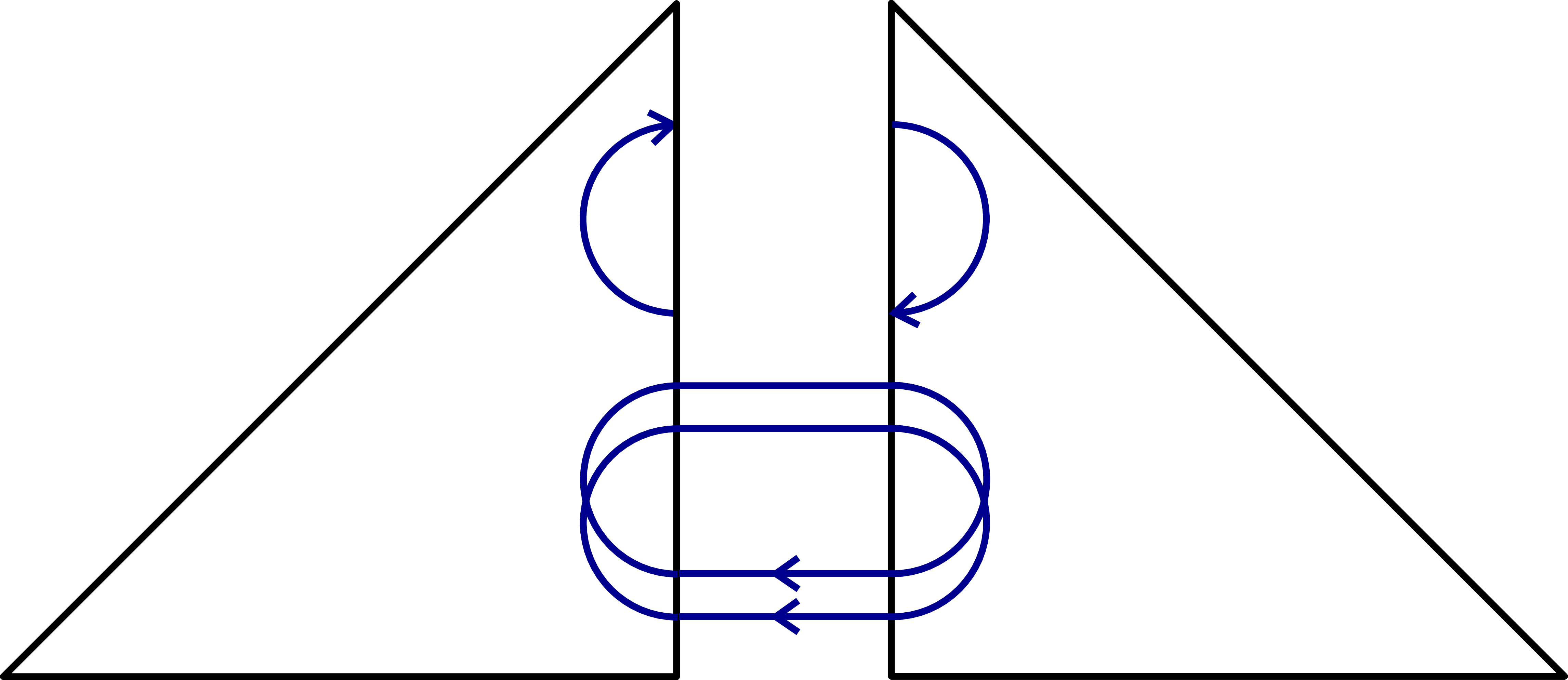
We can map functions from the relaxed \(H(\operatorname{div})\) space to the standard \(H(\operatorname{div})\) space with a very simple average operator (that averages corresponding vector entries):

→

In NGSolve this is easily achieved with calling Average of the relaxed HDiv space:

V.Average(gfu.vec)

A few remarks on the application of the relaxed \(H(\operatorname{div})\)-conforming method:

When applying the relaxed \(H(\operatorname{div})\)-conforming method the velocity solution will in general not be normal-continuous (and thus solenoidal) anymore. With the Average-operator a fully \(H(\operatorname{div})\)-conforming velocity can be postprocessed.
However, to also get “pressure robustness” for the Stokes problem the test function of the r.h.s. linear form needs to apply that average operator as well which is achieved with an application of the Average-operator (a.k.a. reconstruction operator) on the r.h.s. vector.
The relaxed \(H(\operatorname{div})\)-conforming HDG method works nice for the Stokes method and with the Average-operator preserves essentially all properties of the \(H(\operatorname{div})\)-conforming HDG method. However, for Navier-Stokes problems things are a bit more careful (as mass matrix and convection term would in general require the reconstruction operator as well which is algorithmically inconvenient)

Note

For more details on relaxed \(H(\operatorname{div})\)-conforming (H)DG methods see “P.L. Lederer, C. Lehrenfeld and J. Schöberl, Hybrid Discontinuous {Galerkin} methods with relaxed {H(div)}-conformity for incompressible flows. Part I, SINUM, 2018. https://doi.org/10.1137/17M1138078” and “P.L. Lederer, C. Lehrenfeld and J. Schöberl, Hybrid Discontinuous {Galerkin} methods with relaxed {H(div)}-conformity for incompressible flows. Part II, ESAIM: M2AN, 2019. https://doi.org/10.1051/m2an/2018054”

11.5.3. Highest order divergence-free spaces#

The HDiv space in NGSolve has a special construction of the hierarchical bases that allows as to reduce to all basis functions that have a divergence that is orthonal to the constants. For that the flag hodivfree=True can be provided to the FESpace.

When applied in the Stokes system, the pressure (as a Lagrange multiplier for the div-constraint), has to be reduced to piecewise constants in this case.

Note

We note that with the hodivfree-flag only element-bubbles are removed in the velocity and the pressure space, i.e. we only achieve a reduction of LOCAL_DOFs not INTERFACE_DOFs with this approach.

11.5.4. Application to the Stokes discretization#

We take the same geometry as in the previous example:

We consider eight different combination of spaces with three binary decisions:

reduction of the tangential facet space to one order less (or not)
reduction to a relaxed H(div) space with normal continuity only of one degree less (or not)
reduction of interior \(H(div)\) bubbles w.r.t. to the divergence (hodivfree) (or not)

order = 3

VT1 = HDiv(mesh,order=order, dirichlet="top|bottom|side")
VT2 = HDiv(mesh,order=order, dirichlet="top|bottom|side", hodivfree = True )
VT3 = HDiv(mesh,order=order, dirichlet="top|bottom|side", highest_order_dc=True)
VT4 = HDiv(mesh,order=order, dirichlet="top|bottom|side", hodivfree = True, highest_order_dc=True)
Vhat1 = TangentialFacetFESpace(mesh,order=order, dirichlet="bottom|top")
Vhat2 = Compress(TangentialFacetFESpace(mesh,order=order, dirichlet="bottom|top", highest_order_dc=True, hide_highest_order_dc=True))
Q1 = L2(mesh,order=order-1, lowest_order_wb=True)
Q2 = L2(mesh,order=0, lowest_order_wb=True)
N = NumberSpace(mesh)
fes_params= [(VT1,Vhat1,Q1,"std"), \
             (VT1,Vhat2,Q1,"t. red."), \
             (VT3,Vhat1,Q1,"n. red."), \
             (VT3,Vhat2,Q1,"n.+t. red."), \
             (VT2,Vhat1,Q2,"            hodf"), \
             (VT2,Vhat2,Q2,"t. red.,    hodf"), \
             (VT4,Vhat1,Q2,"n. red.,    hodf"), \
             (VT4,Vhat2,Q2,"n.+t. red., hodf")]
labeled_fes = [(VT * Vhat * Q * N, name) for VT,Vhat,Q,name in fes_params]

We setup the HDG Stokes system:

def setup_Stokes_HDG_system(fes, **opts):
    nu = 1
    gamma = 10
    yh, zh = fes.TnT()
    order = fes.components[0].globalorder
    (u, uhat, p, lam), (v, vhat, q, mu) = yh, zh
    uh, vh = (u, uhat), (v, vhat)
    tang = lambda u: u - (u*n)*n
    tjump = lambda uh: tang(uh[0]-uh[1]) 

    n = specialcf.normal(mesh.dim)
    h = specialcf.mesh_size

    K = BilinearForm(fes, **opts)
    K += (nu*InnerProduct(Grad(u), Grad(v)) + div(u)*q + div(v)*p + p * mu + q * lam) * dx
    K += nu * Grad(u) * n * tjump(vh) * dx(element_boundary = True)
    K += nu * Grad(v) * n * tjump(uh) * dx(element_boundary = True)
    K += nu  *gamma*order**2/h * InnerProduct ( tjump(vh),  tjump(uh) ) * dx(element_boundary = True)
    K.Assemble()

    r = sqrt(x**2+y**2)
    f = LinearForm(fes)
    f += 500*CF((0,0,r-0.5))*v*dx
    f.Assemble()

    fes.components[0].Average(f.vec)

    return K,f

For different options on how to eliminate dofs and for the different methods we compute some metrics of the solution of the resulting linear systems: Effectively for every combination of methods we call:

a,f = setup_Stokes_HDG_system(fes, ...)
solve_lin_system(a,f, gfu=gfu)

Show code cell source Hide code cell source

linsys_opts = [({"condense": False},"  none"), \
               ({"eliminate_hidden": True},"hidden"), \
               ({"condense": True}," local")]
import time
try:
  import pandas as pd
  from IPython.display import display, HTML
  html_output = True
except:
  html_output = False
data = []
with TaskManager():
  for opts, elims in linsys_opts:
    if not html_output:
      print(f"\n\n dof elimination: {elims:9} \n")
      print(f"                |           ndofs          | ncdofs |     nze  | timing (ass.+sol.)")
      print(f"----------------|--------------------------|--------|----------|-------------------")    
    for fes, label in labeled_fes:
      gfu = GridFunction(fes)
      gfu.components[1].Set(CF((y,-x,0)), definedon=mesh.Boundaries("bottom"))
      timer1 = time.time()
      a,f = setup_Stokes_HDG_system(fes, **opts)
      timer2 = time.time()
      solve_lin_system(a,f, gfu=gfu)
      timer3 = time.time()
      if html_output:
        data.append([elims,label,fes.ndof,fes.components[0].ndof,fes.components[1].ndof,
                     fes.components[2].ndof,fes.components[3].ndof,
                     sum(fes.FreeDofs(coupling=True)),
                     "{:.0f}K".format(a.mat.nze/1000),"{:5.3f}".format(timer3-timer1),
                     "{:5.3f}".format(timer2-timer1),"{:5.3f}".format(timer3-timer2)])
      else:
        print(f"{label:16}|",end="")
        print(f"{fes.ndof:5}({fes.components[0].ndof:5}+{fes.components[1].ndof:5}",end="")
        print(f"{fes.components[2].ndof:5}+{fes.components[3].ndof:1})",end=" ")
        print(f"|{sum(fes.FreeDofs(coupling=True)):7}", end=" ")
        print(f"|{a.mat.nze:9}", end=" ")
        print(f"| {timer3-timer1:4.2f} = {timer2-timer1:4.2f} + {timer3-timer2:4.2f}")
if not html_output:
  print(f"----------------|--------------------------|--------|----------|-------------------")
  print("")
else:
  display(HTML(pd.DataFrame(data, 
                            columns=["dof elim.", "FESpace", "ndofs", "nd0", "nd1", 
                                     "nd2", "nd3","ncdofs","nze","time","ass.",
                                     "sol."]).to_html(border=0,index=False)))                     

dof elim.	FESpace	ndofs	nd0	nd1	nd2	nd3	ncdofs	nze	time	ass.	sol.
none	std	25501	10980	12040	2480	1	13589	5280K	0.918	0.076	0.842
none	t. red.	20685	10980	7224	2480	1	9813	3306K	0.883	0.141	0.743
none	n. red.	27061	12540	12040	2480	1	12029	5370K	0.946	0.128	0.817
none	n.+t. red.	22245	12540	7224	2480	1	8253	3371K	0.552	0.115	0.438
none	hodf	21037	8748	12040	248	1	13589	4012K	0.601	0.113	0.488
none	t. red., hodf	16221	8748	7224	248	1	9813	2324K	0.449	0.141	0.308
none	n. red., hodf	22597	10308	12040	248	1	12029	4103K	0.625	0.074	0.551
none	n.+t. red., hodf	17781	10308	7224	248	1	8253	2389K	0.424	0.054	0.370
hidden	std	25501	10980	12040	2480	1	13589	5280K	0.837	0.100	0.737
hidden	t. red.	20685	10980	7224	2480	1	9813	3306K	0.585	0.077	0.508
hidden	n. red.	27061	12540	12040	2480	1	12029	5370K	0.841	0.092	0.748
hidden	n.+t. red.	22245	12540	7224	2480	1	8253	3371K	0.523	0.086	0.437
hidden	hodf	21037	8748	12040	248	1	13589	4012K	0.667	0.094	0.574
hidden	t. red., hodf	16221	8748	7224	248	1	9813	2324K	0.440	0.102	0.337
hidden	n. red., hodf	22597	10308	12040	248	1	12029	4103K	0.707	0.087	0.621
hidden	n.+t. red., hodf	17781	10308	7224	248	1	8253	2389K	0.344	0.057	0.287
local	std	25501	10980	12040	2480	1	13589	3317K	0.499	0.099	0.400
local	t. red.	20685	10980	7224	2480	1	9813	1803K	0.351	0.096	0.255
local	n. red.	27061	12540	12040	2480	1	12029	2687K	0.633	0.186	0.447
local	n.+t. red.	22245	12540	7224	2480	1	8253	1348K	0.289	0.132	0.158
local	hodf	21037	8748	12040	248	1	13589	3317K	0.737	0.175	0.562
local	t. red., hodf	16221	8748	7224	248	1	9813	1803K	0.426	0.208	0.218
local	n. red., hodf	22597	10308	12040	248	1	12029	2687K	0.590	0.145	0.445
local	n.+t. red., hodf	17781	10308	7224	248	1	8253	1348K	0.500	0.159	0.341

Warning

The combination of tang. red and no condensation (condensed dofs: none) will not yield reasonable numerical results, see discussion above.

Let us check if the most reduced solution space (which yields the cheapest solution) is still able to solve the problem, by inspecting the solution:

N = 15
points = [ (sin(2*pi*k/N)*i/N, cos(2*pi*k/N)*i/N, j/N)   for i in range(1,N) for j in range(1,N) for k in range(0,N)]
fl = gfu.components[0]._BuildFieldLines(mesh, points, num_fieldlines=N**3//20, randomized=True, length=1)
ea = { "euler_angles" : (-40, 0, 0) }
Draw(gfu.components[0], mesh,  "X", draw_vol=False, draw_surf=True, objects=[fl], \
     min=0, max=1, autoscale=False, settings={"Objects": {"Surface": False, "Wireframe":False}}, **ea);

Normal-cont. HDG tricks

Contents

11.5. Normal-cont. HDG tricks#

11.5.1. Projected jumps for the TangentialFacetFESpace#

11.5.2. Relaxed \(H(\operatorname{div})\)-conforming FESpaces#

11.5.3. Highest order divergence-free spaces#

11.5.4. Application to the Stokes discretization#

11.5.1. Projected jumps for the `TangentialFacetFESpace`#

11.5.2. Relaxed \(H(\operatorname{div})\)-conforming `FESpace`s#