6.1. Linear elasticity#
from netgen.occ import *
from ngsolve import *
from ngsolve.webgui import Draw
from netgen.webgui import Draw as DrawGeo
The body of interest
box = Box((0,0,0), (3,0.6,1))
box.faces.name="outer"
cyl = sum( [Cylinder((0.5+i,0,0.5), Y, 0.25,0.8) for i in range(3)] )
cyl.faces.name="cyl"
geo = box-cyl
ea = { "euler_angles" : [-70,5,30] }
cylboxedges = geo.faces["outer"].edges * geo.faces["cyl"].edges
cylboxedges.name = "cylbox"
geo = geo.MakeChamfer(cylboxedges, 0.03)
geo.faces.Min(X).name = "fix"
geo.faces.Max(X).name = "force"
Draw(geo, **ea)
mesh = Mesh(OCCGeometry(geo).GenerateMesh(maxh=0.1)).Curve(3)
scene = Draw (mesh, **ea)
6.1.1. Linear elasticity in local form#
Displacement: \(\vec u : \Omega \rightarrow {\mathbb R}^3\)
Linear strain:
Linear isotropic material: linear stress/strain relation for the symmetric stress tensor \(\boldsymbol \sigma\), Hooke’s law
Equilibrium of forces:
Displacement boundary conditions:
Traction boundary conditions for the stress vector \(\boldsymbol \sigma \cdot \vec n\)
6.1.2. Variational formulation:#
Find: \(\vec u \in H^1(\Omega)^3\) such that \(\vec u = \vec u_D\) on \(\Gamma_D\) and
holds for all \(\vec v\) with \(\vec v = 0\) on \(\Gamma_D\).
E, nu = 210, 0.2
mu = E / 2 / (1+nu)
lam = E * nu / ((1+nu)*(1-2*nu))
def Stress(strain):
return 2*mu*strain + lam*Trace(strain)*Id(3)
fes = VectorH1(mesh, order=3, dirichlet="fix")
u,v = fes.TnT()
gfu = GridFunction(fes)
with TaskManager():
a = BilinearForm(InnerProduct(Stress(Sym(Grad(u))), Sym(Grad(v))).Compile()*dx)
pre = Preconditioner(a, "bddc")
a.Assemble()
force = CF( (1e-3,0,0) )
f = LinearForm(force*v*ds("force")).Assemble()
from ngsolve.krylovspace import CGSolver
inv = CGSolver(a.mat, pre, tol=1e-8)
gfu.vec.data = inv * f.vec
Postprocessing for the stresses:
with TaskManager():
fesstress = MatrixValued(H1(mesh,order=3), symmetric=True)
gfstress = GridFunction(fesstress)
gfstress.Interpolate (Stress(Sym(Grad(gfu))))
Visualization: visualize the displacement vector on the deformed geometry, use “deformation” slider for scaling
Draw (gfu, mesh, deformation=True, scale=3e4, **ea)
BaseWebGuiScene
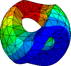
Visualize the stress norm \(|\boldsymbol \sigma|\) on the deformed geometry.
Draw (Norm(gfstress), mesh, deformation=1e4*gfu, draw_vol=False, order=3, **ea)
BaseWebGuiScene
6.1.3. The principle of virtual work#
The variational formulation is well-known as principle of virtual work: For all kinematicall admissible virtual displacements \(\delta \vec u\) (i.e. \(\delta \vec u \in H^1(\Omega)^3\) with \(\delta \vec u = \vec 0\) on \(\Gamma_D\)), the virtual work of internal forces equals the virtual work of external forces.
The virtual work of internal forces can be defined conveniently using the energy density \(\psi\) of the material. For
we get the left hand side of the variational equation via
The right hand side corresponds to the virtual work of external forces,
Both contributions can be collected in the bilinear form; for the virtual work of internal forces, Variation allows to put the elastic energy explicitely and let ngsolve do the differentiation. For the virtual work of external forces, both an implementation via Variation (for conservative forces) or via a work statement is possible. AssembleLinearization generates the stiffness matrix, Apply the residual vector.
Use this approach below:
fes = VectorH1(mesh, order=3, dirichlet="fix")
u, deltau = fes.TnT()
gfu = GridFunction(fes)
def psi(u):
strain = Sym(Grad(u))
return mu*InnerProduct(strain,strain) + lam/2*Trace(strain)**2
a = BilinearForm(fes, symmetric=True)
a += Variation(psi(u)*dx)
a += -force*deltau*ds("force")
with TaskManager():
a.AssembleLinearization(gfu.vec)
res = gfu.vec.CreateVector()
a.Apply(gfu.vec, res)
inv = a.mat.Inverse(fes.FreeDofs())
gfu.vec.data -= inv * res
The solution is, of course, equivalent to the one above.
Exercise:
apply loading in \(z\)-direction.
look at individual components of stress-tensor (like
gfstress[0,0])apply a volume load \(\vec f\) instead of the surface load
