Linear and nonlinear shell models

9.1. Linear and nonlinear shell models#

In this section we will motivate and discuss different shell models, namely,

Nonlinear Naghdi shell
Nonlinear Koiter shell
Linear Reissner-Mindlin shell
Linear Kirchhoff-Love shell

We will focus on the different energies arising in these models. For a comprehensive introduction and derivation to shell models we refer to the literature, e.g.

9.1.1. Notation#

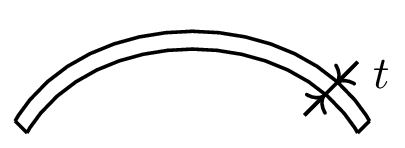
We call three-dimensional objects \(\Omega\subset\mathbb{R}^3\), where one direction is significantly smaller than the others, thin-walled structures. Examples are parts of cars and air planes, or cell membranes. Discretizing them fully would lead to a vast amount of elements, which is rather inefficient. Therefore a dimension reduction is made by only considering the mid-surface \(\mathcal{S}\) of the structure and its thickness \(t\). This is motivated as we can describe each point of \(\Omega\) in the following form (for small enough \(t\))

\[\begin{align*} \Omega=\left\{\xi+z\hat{\nu}(\xi):\, \xi\in \mathcal{S}, z\in \left[-\frac{t}{2},\frac{t}{2}\right]\right\}, \end{align*}\]

where \(\hat{\nu}\) is the normal vector on the mid-surface \(\mathcal{S}\).

Nonlinear Koiter and linear Kirchhoff-Love shells have the displacement field \(u:\mathcal{S}\to\mathbb{R}^3\) of the mid-surface as primary unknown. Models where also rotation or shearing is used as additional unknowns are frequently called nonlinear Nagdhi and linear Reissner-Mindlin shells.

Analogously to continuum mechanics we define the (surface) deformation gradient \(F_{\mathcal{S}}=P_{\mathcal{S}}+\nabla_{\mathcal{S}}u\), where in contrast to elasticity (\(F=I+\nabla u\)) the surface gradient \(\nabla_{\mathcal{S}}u\) has to be used and the projection onto the surface \(P_{\mathcal{S}} = I -\hat{\nu}\otimes\hat{\nu}\) as we are only on the surface and not in the full space. The surface Cauchy-Green and surface Green strain tensors are then given by

\[\begin{align*} C_{\mathcal{S}} = F_{\mathcal{S}}^\top F_{\mathcal{S}},\qquad E_{\mathcal{S}}=\frac{1}{2}(C_{\mathcal{S}}-P_{\mathcal{S}}). \end{align*}\]

We will motivate the different energy terms of a shell: Membrane, bending, and shearing energy.

9.1.2. Membrane energy#

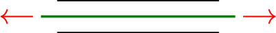
The membrane energy measures how much the mid-surface gets stretched. This is given by the deviation of the Cauchy-Green strain tensor from the identity tensor of the surface, i.e., the surface Green strain tensor \(E_{\mathcal{S}}\)

\[\begin{align*} \mathcal{W}_{\mathrm{mem}}(u)= \frac{t}{2}\int_{\mathcal{S}}\|E_{\mathcal{S}}\|^2_{\mathbb{C}}\,ds, \end{align*}\]

where \(\mathbb{C}\) denotes the material tensor being commonly of the form

\[\begin{align*} \mathbb{C} E_{\mathcal{S}} = \frac{\bar E}{1-\bar \nu^2}\big((1-\bar \nu)E_{\mathcal{S}}+\bar \nu\,\mathrm{tr}(E_{\mathcal{S}})P_{\mathcal{S}}\big), && \|E_{\mathcal{S}}\|^2_{\mathbb{C}} = (\mathbb{C}E_{\mathcal{S}}):E_{\mathcal{S}}, \end{align*}\]

where \(\bar E\) and \(\bar \nu\) denote the Young modulus and Poisson ratio, respectively, and classically the plain stress assumption is assumed (no stress in thickness direction). The linear scaling of the thickness \(t\) can be derived e.g. by asymptotic analysis starting from 3D elasticity.

from ngsolve import *
from ngsolve.webgui import Draw
from netgen.occ import *

mesh = Mesh(OCCGeometry(Rectangle(1, 1).Face()).GenerateMesh(maxh=0.2))
gfu = GridFunction(VectorH1(mesh, order=3))

# unit normal vector of the surface
nsurf = specialcf.normal(3)
# projection onto the surface
Ptau = Id(3) - OuterProduct(nsurf, nsurf)
F = Grad(gfu) + Ptau
E = 0.5 * (F.trans * F - Ptau)

gfu.Set(
    CF((0.5 * x**2, -0.1 * (y - 0.5) + 0.3 * x, 0)), definedon=mesh.Boundaries(".*")
)

Draw(gfu, mesh, "gfu", deformation=True, euler_angles=[-30, 0, 0])
Draw(E[0, 0], mesh, "Exx");

9.1.3. Bending energy#

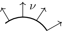
The bending energy measures the difference of the curvatures between the initial and deformed configuration. The curvature of a surface can by computed by the Weingartentensor (also called shape operator), which is the surface gradient of the normal vector \(\nu\) of the surface, \(\nabla_{\mathcal{S}}\nu\). From it we can compute the mean curvature \(H\) and Gauss curvature \(K\) of the surface.

E.g., for a cylindrical geometry (\(H=\frac{1}{2r}\), \(K=0\))

cyl = Cylinder((0, 0, 0), (1, 0, 0), r=1, h=3).faces[0]
mesh = Mesh(OCCGeometry(cyl).GenerateMesh(maxh=0.2)).Curve(5)

Draw(Grad(nsurf)[1, 1], mesh, "Weingarten_yy", euler_angles=[0, -50, -10])
Draw(
    0.5 * Trace(Grad(nsurf)),
    mesh,
    "mean_curvature",
    min=0.45,
    max=0.55,
    euler_angles=[0, -50, -10],
)
Draw(
    Norm(Cof(Grad(nsurf))),
    mesh,
    "Gauss_curvature",
    min=-1,
    max=1,
    euler_angles=[0, -50, -10],
);

or a sphere (\(H=\frac{1}{r}\), \(K=\frac{1}{r^2}\))

mesh = Mesh(OCCGeometry(Sphere((0, 0, 0), r=2)).GenerateMesh(maxh=0.2)).Curve(5)

Draw(0.5 * Trace(Grad(nsurf)), mesh, "mean_curvature")
Draw(Norm(Cof(Grad(nsurf))), mesh, "Gauss_curvature");

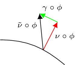
The bending energy of the shell is given by

\[\begin{align*} \mathcal{W}_{\mathrm{bend}}(u) &=\frac{t^3}{24}\int_{\mathcal{S}}\|F_{\mathcal{S}}^\top\nabla_{\mathcal{S}}(\nu\circ\phi)-\nabla_{\mathcal{S}}\hat{\nu}\|^2_{\mathbb{C}}\,ds \\ &= \frac{t^3}{24}\int_{\mathcal{S}}\Big\|\sum_{i=1}^3(\nabla_{\mathcal{S}}^2u_i)(\nu\circ\phi)_i+(1- \hat{\nu}\cdot\nu\circ\phi)\nabla_{\mathcal{S}}\hat{\nu}\Big\|^2_{\mathbb{C}}\,ds, \end{align*}\]

where \(\hat{\nu}\) is the normal vector of the initial shell, \(\nu\circ\phi=\frac{1}{\|\mathrm{cof}(F_{\mathcal{S}})\hat{\nu}\|}\mathrm{cof}(F_{\mathcal{S}})\hat{\nu}\) the normal vector on the deformed shell \(\tilde{\mathcal{S}}=\phi(\mathcal{S})\), and \(\nabla_{\mathcal{S}}^2u_i\) denotes the surface Hessian.

mesh = Mesh(OCCGeometry(Rectangle(1, 1).Face()).GenerateMesh(maxh=0.2))

gfu = GridFunction(VectorH1(mesh, order=6))

F = Grad(gfu) + Ptau
E = 0.5 * (F.trans * F - Ptau)

# factor = 1 -> no membrane energy; factor = pi/2 -> non-zero membrane energy
factor = 1  # pi/2
gfu.Set(
    CF((-x + sin(factor * x), 0, -cos(factor * x) + 1)), definedon=mesh.Boundaries(".*")
)
Draw(gfu, mesh, "gfu", deformation=True, euler_angles=[-30, 0, 0])
Draw(Norm(E), mesh, "membrane_energy", max=1e-8)

nphys = Normalize(Cof(F) * nsurf)
bending_term = (gfu.Operator("hesseboundary", BND).trans * nphys).Reshape((3, 3)) + (
    1 - nsurf * nphys
) * Grad(nsurf)

Draw(
    Norm(bending_term),
    mesh,
    "bending_energy",
    min=factor**2 - 1e-4 * factor,
    max=factor**2 + 1e-4 * factor,
);

9.1.4. Shearing energy#

For nonlinear Koiter and linear Kirchhoff-Love shells by assumption there is no shearing energy, it is zero. Nonlinear Naghdi and linear Reissner-Mindlin shells, however, extend the Koiter/Kirchhoff-Love shell models by including a possible shear \(\gamma\) of the normal vectors.

The shear energy measures how strong the new so-called ‘’director’’ \(\tilde{\nu}\circ\phi\) differs from being perpendicular to the mid-surface of the deformed shell

\[\begin{align*} \mathcal{W}_{\mathrm{shear}}(u,\gamma) = \frac{tG\kappa}{2}\|F_{\mathcal{S}}^\top\tilde{\nu}\circ\phi\|^2, \end{align*}\]

where \(G=\frac{E}{2(1+\nu)}\) denotes the shearing modulus and \(\kappa=\frac{5}{6}\) the so-called shear correction factor. Note, that the director \(\tilde{\nu}\) is used in the bending energy term.

If the thickness is very small the shear energy might be neglectable, but for bigger values of \(t\) including the shear term can increase the accuracy of the shell model.

9.1.5. Total nonlinear Koiter and Naghdi shell energies#

Summing up, the total shell energy for a Naghdi shell (including shearing) reads

\[\begin{align*} \mathcal{W}_{\mathrm{Naghdi}}(u,\gamma)&=\mathcal{W}_{\mathrm{mem}}(u)+\mathcal{W}_{\mathrm{bend}}(u,\gamma) +\mathcal{W}_{\mathrm{shear}}(u,\gamma) - \int_{\mathcal{S}}f\cdot u\,ds\\ &= \int_{\mathcal{S}}\Big(\frac{t}{2}\|E_{\mathcal{S}}\|^2_{\mathbb{C}}+\frac{t^3}{24}\|F_{\mathcal{S}}^\top\nabla_{\mathcal{S}}(\tilde \nu\circ\phi)-\nabla_{\mathcal{S}}\hat{\nu}\|^2_{\mathbb{C}} +\frac{tG\kappa}{2}\|F_{\mathcal{S}}^\top\tilde{\nu}\circ\phi\|^2\Big)\,ds - \int_{\mathcal{S}}f\cdot u\,ds \end{align*}\]

and for the Koiter shell model is given by

\[\begin{align*} \mathcal{W}_{\mathrm{Koiter}}(u)&=\mathcal{W}_{\mathrm{mem}}(u)+\mathcal{W}_{\mathrm{bend}}(u) - \int_{\mathcal{S}}f\cdot u\,ds\\ &= \int_{\mathcal{S}}\Big(\frac{t}{2}\|E_{\mathcal{S}}\|^2_{\mathbb{C}}+\frac{t^3}{24}\|F_{\mathcal{S}}^\top\nabla_{\mathcal{S}}(\nu\circ\phi)-\nabla_{\mathcal{S}}\hat{\nu}\|^2_{\mathbb{C}}\Big)\,ds - \int_{\mathcal{S}}f\cdot u\,ds. \end{align*}\]

9.1.6. Linear Kirchhoff-Love and Reissner-Mindlin shells#

By applying the small-strain assumption, we can linearize the nonlinear shell models to obtain their linear counter-parts. The linear Kirchhoff-Love shell reads

\[\begin{align*} \mathcal{W}_{\mathrm{KL}}(u)=\int_{\mathcal{S}}\Big(\frac{t}{2}\|\mathrm{sym}(\nabla_{\mathcal{S}}^{\mathrm{cov}}u)\|^2_{\mathbb{C}} + \frac{t^3}{24}\Big\|\sum_{i=1}^3\nabla_{\mathcal{S}}^2u_i \nu_i\Big\|^2_{\mathbb{C}}\Big)\,ds - \int_{\mathcal{S}}f\cdot u\,ds, \end{align*}\]

where \(\nabla_{\mathcal{S}}^{\mathrm{cov}}=P_{\mathcal{S}}\nabla_{\mathcal{S}}\) is the covariant derivative and the linear Reissner-Mindlin shell

\[\begin{align*} \mathcal{W}_{\mathrm{RM}}(u,\gamma)=\int_{\mathcal{S}}\Big(\frac{t}{2}\|\mathrm{sym}(\nabla_{\mathcal{S}}^{\mathrm{cov}}u)\|^2_{\mathbb{C}} + \frac{t^3}{24}\Big\|\sum_{i=1}^3\nabla_{\mathcal{S}}^2u_i \nu_i-\nabla_{\mathcal{S}}\gamma\Big\|^2_{\mathbb{C}} + \frac{t\kappa G}{2}\|\gamma\|_2\Big)\,ds - \int_{\mathcal{S}}f\cdot u\,ds. \end{align*}\]

9.1.7. Reduction to linear plates#

Assuming that the initial configuration of the shell is a plate, the membrane energy decouples from the bending and shearing energies. Therefore, the linear Kirchhoff-Love and Reissner-Mindlin shells reduce to the well known Kirchhoff-Love and Reissner-Mindlin plate models

\[\begin{align*} \mathcal{W}_{\mathrm{KL,plate}}(u)&=\int_{\mathcal{S}} \frac{t^3}{24}\|\nabla^2w \|^2_{\mathbb{C}}\,ds -\int_{\mathcal{S}} f\cdot u\,ds,\\ \mathcal{W}_{\mathrm{RM,plate}}(u,\beta)&=\int_{\mathcal{S}} \Big(\frac{t^3}{24}\|\mathrm{sym}(\nabla\beta)\|^2_{\mathbb{C}} + \frac{t\kappa G}{2}\|\nabla w-\beta\|_2\Big)\,ds - \int_{\mathcal{S}}f\cdot u\,ds, \end{align*}\]

where we used the change of variable \(\beta = \nabla w-\gamma\) from a shearing \(\gamma\) to a rotation \(\beta\) field.

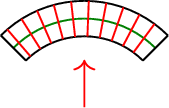
9.1.8. Challenge: Affine triangulation for Koiter shells#

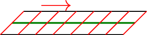
What happens for the bending energy if we consider only a linear triangulation and a linear displacement \(u\) field? It is zero element-wise as the unit normal vector is constant on each triangle!

Each triangle is flat and gets deformed linearly such that the deformed triangle is still flat. Thus, no change of curvature is measured.

Question: So how to treat the curvature in this case?

Answer: Look at discrete differential geometry!

The curvature information sits only at the edges: The angle between the normal vectors tells us how strong the geometry is curved!

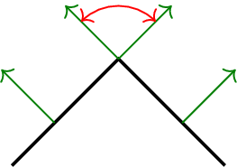
So we should measure the change of curvature by the change of angles in this case

\[\begin{align*} \mathcal{W}_{\mathrm{bend}}^{\mathrm{new}}(u) =\frac{t^3}{24}\sum_{\mathrm{edges}}\|\sphericalangle(\nu_L,\nu_R)-\sphericalangle(\hat{\nu}_L,\hat{\nu}_R)\|_{\mathbb{C}}. \end{align*}\]

We will incorporate this idea in terms of the HHJ method allowing for affine, unstructured triangular grids also for nonlinear Koiter shells.