This page was generated from unit-2.1.4-bddc/bddc.ipynb.
2.1.4 Element-wise BDDC Preconditioner
The element-wise BDDC (Balancing Domain Decomposition preconditioner with Constraints) preconditioner in NGSolve is a good general purpose preconditioner that works well both in the shared memory parallel mode as well as in distributed memory mode. In this tutorial, we discuss this preconditioner, related built-in options, and customization from python.
Let us start with a simple description of the element-wise BDDC in the context of Lagrange finite element space \(V\). Here the BDDC preconditioner is constructed on an auxiliary space \(\widetilde{V}\) obtained by connecting only element vertices (leaving edge and face shape functions discontinuous). Although larger, the auxiliary space allows local elimination of edge and face variables. Hence an analogue of the original matrix \(A\) on this space, named \(\widetilde A\), is less expensive to invert. This inverse is used to construct a preconditioner for \(A\) as follows:
Here, \(R\) is the averaging operator for the discontinuous edge and face variables.
To construct a general purpose BDDC preconditioner, NGSolve generalizes this idea to all its finite element spaces by a classification of degrees of freedom. Dofs are classified into (condensable) LOCAL_DOFs that we saw in 1.4 and a remainder that includes these types:
WIREBASKET_DOFINTERFACE_DOFThe original finite element space \(V\) is obtained by requiring conformity of both the above types of dofs, while the auxiliary space \(\widetilde{V}\) is obtained by requiring conformity of WIREBASKET_DOFs only.
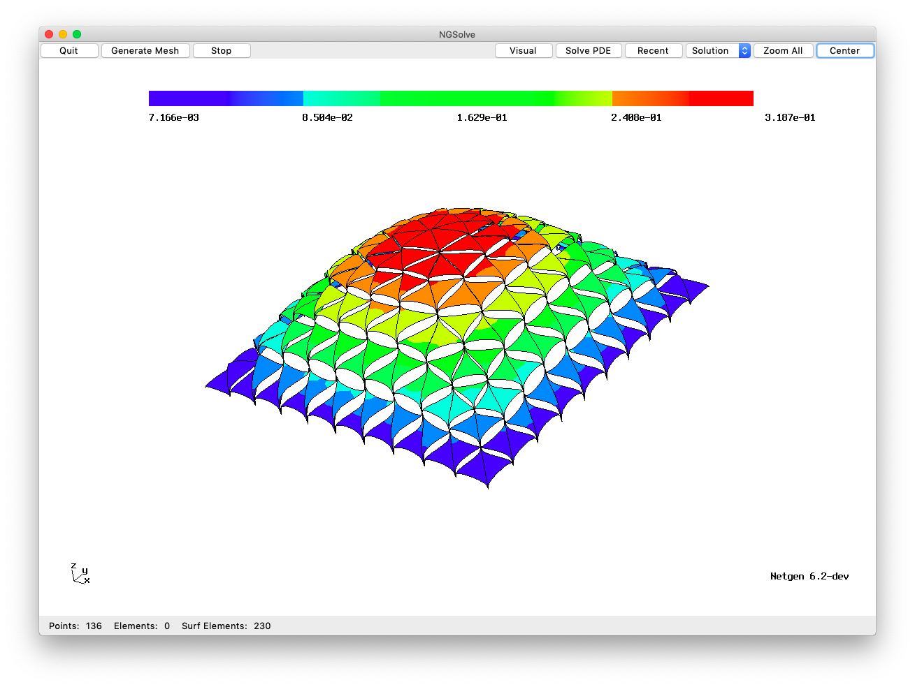
Here is a figure of a typical function in the default \(\widetilde{V}\) (and the code to generate this is at the end of this tutorial) when \(V\) is the Lagrange space:
[1]:
from ngsolve import *
from ngsolve.webgui import Draw
from ngsolve.la import EigenValues_Preconditioner
SetHeapSize(100*1000*1000)
[2]:
mesh = Mesh(unit_cube.GenerateMesh(maxh=0.5))
# mesh = Mesh(unit_square.GenerateMesh(maxh=0.5))
Built-in options
Let us define a simple function to study how the spectrum of the preconditioned matrix changes with various options.
Effect of condensation
[3]:
def TestPreconditioner (p, condense=False, **args):
fes = H1(mesh, order=p, **args)
u,v = fes.TnT()
a = BilinearForm(fes, eliminate_internal=condense)
a += grad(u)*grad(v)*dx + u*v*dx
c = Preconditioner(a, "bddc")
a.Assemble()
return EigenValues_Preconditioner(a.mat, c.mat)
[4]:
lams = TestPreconditioner(5)
print (lams[0:3], "...\n", lams[-3:])
1.00052
1.03338
1.09991
...
4.55515
4.60067
4.79194
Here is the effect of static condensation on the BDDC preconditioner.
[5]:
lams = TestPreconditioner(5, condense=True)
print (lams[0:3], "...\n", lams[-3:])
1.00023
1.02753
1.08363
...
4.06546
4.12581
4.22957
Tuning the auxiliary space
Next, let us study the effect of a few built-in flags for finite element spaces that are useful for tweaking the behavior of the BDDC preconditioner. The effect of these flags varies in two (2D) and three dimensions (3D), e.g.,
wb_fulledges=True: This option keeps all edge-dofs conforming (i.e. they are markedWIREBASKET_DOFs). This option is only meaningful in 3D. If used in 2D, the preconditioner becomes a direct solver.wb_withedges=True: This option keeps only the first edge-dof conforming (i.e., the first edge-dof is markedWIREBASKET_DOFand the remaining edge-dofs are markedINTERFACE_DOFs).
The complete situation is a bit more complex due to the fact these options can take the three values True, False, or Undefined, the two options can be combined, and the space dimension can be 2 or 3. The default value of these flags in NGSolve is Undefined. Here is a table with the summary of the effect of these options:
wb_fulledges |
wb_withedges |
2D |
3D |
|---|---|---|---|
True |
any value |
all |
all |
False/Undefined |
Undefined |
none |
first |
False/Undefined |
False |
none |
none |
False/Undefined |
True |
first |
first |
An entry \(X \in\) {all, none, first} of the last two columns is to be read as follows: \(X\) of the edge-dofs is(are) WIREBASKET_DOF(s).
Here is an example of the effect of one of these flag values.
[6]:
lams = TestPreconditioner(5, condense=True,
wb_withedges=False)
print (lams[0:3], "...\n", lams[-3:])
1.00106
1.07035
1.22031
...
25.4058
25.406
26.9095
Clearly, when moving from the default case (where the first of the edge dofs are wire basket dofs) to the case (where none of the edge dofs are wire basket dofs), the conditioning became less favorable.
Customize
From within python, we can change the types of degrees of freedom of finite element spaces, thus affecting the behavior of the BDDC preconditioner.
To depart from the default and commit the first two edge dofs to wire basket, we perform the next steps:
[7]:
fes = H1(mesh, order=10)
u,v = fes.TnT()
for ed in mesh.edges:
dofs = fes.GetDofNrs(ed)
for d in dofs:
fes.SetCouplingType(d, COUPLING_TYPE.INTERFACE_DOF)
# Set the first two edge dofs to be conforming
fes.SetCouplingType(dofs[0], COUPLING_TYPE.WIREBASKET_DOF)
fes.SetCouplingType(dofs[1], COUPLING_TYPE.WIREBASKET_DOF)
a = BilinearForm(fes, eliminate_internal=True)
a += grad(u)*grad(v)*dx + u*v*dx
c = Preconditioner(a, "bddc")
a.Assemble()
lams=EigenValues_Preconditioner(a.mat, c.mat)
max(lams)/min(lams)
[7]:
9.989385160527968
This is a slight improvement from the default.
[8]:
lams = TestPreconditioner (10, condense=True)
max(lams)/min(lams)
[8]:
13.974958344241063
Combine BDDC with AMG for large problems
coarsetype=h1amg flag, we can ask BDDC to replace \({\,\widetilde{A}\,}^{-1}\) by an Algebraic MultiGrid (AMG) preconditioner. Since NGSolve’s h1amg is well-suitedwb_withedges=False to ensure that \(\widetilde{A}\) is made solely with vertex unknowns.[9]:
p = 5
mesh = Mesh(unit_cube.GenerateMesh(maxh=0.05))
fes = H1(mesh, order=p, dirichlet="left|bottom|back",
wb_withedges=False)
print("NDOF = ", fes.ndof)
u,v = fes.TnT()
a = BilinearForm(fes)
a += grad(u)*grad(v)*dx
f = LinearForm(fes)
f += v*dx
with TaskManager():
pre = Preconditioner(a, "bddc", coarsetype="h1amg")
a.Assemble()
f.Assemble()
gfu = GridFunction(fes)
solvers.CG(mat=a.mat, rhs=f.vec, sol=gfu.vec,
pre=pre, maxsteps=500)
Draw(gfu)
NDOF = 746336
CG iteration 1, residual = 0.7291770014214167
CG iteration 2, residual = 0.30858257666351824
CG iteration 3, residual = 0.27517322278059086
CG iteration 4, residual = 0.3147145873897679
CG iteration 5, residual = 0.32591310046285565
CG iteration 6, residual = 0.235765045826115
CG iteration 7, residual = 0.1939850925872334
CG iteration 8, residual = 0.17172300961311635
CG iteration 9, residual = 0.1285987335654353
CG iteration 10, residual = 0.0937315719812052
CG iteration 11, residual = 0.06655712957878444
CG iteration 12, residual = 0.05174938893736048
CG iteration 13, residual = 0.041724157511087136
CG iteration 14, residual = 0.03202349002517119
CG iteration 15, residual = 0.024269037283164076
CG iteration 16, residual = 0.018659350366406386
CG iteration 17, residual = 0.014925202785173466
CG iteration 18, residual = 0.01146551505523322
CG iteration 19, residual = 0.008563421986446686
CG iteration 20, residual = 0.006510717807331401
CG iteration 21, residual = 0.004990438762243244
CG iteration 22, residual = 0.003885537772119369
CG iteration 23, residual = 0.002883633564280215
CG iteration 24, residual = 0.0021959004578735674
CG iteration 25, residual = 0.0016985067526936876
CG iteration 26, residual = 0.0013046513241761126
CG iteration 27, residual = 0.0010193922821228486
CG iteration 28, residual = 0.0007914753128941833
CG iteration 29, residual = 0.0006101146090473376
CG iteration 30, residual = 0.00046837780626702316
CG iteration 31, residual = 0.00036001775986599865
CG iteration 32, residual = 0.00027050038473704085
CG iteration 33, residual = 0.00020840288233808793
CG iteration 34, residual = 0.00016312242859642373
CG iteration 35, residual = 0.00012581238102933118
CG iteration 36, residual = 0.00010118196850657358
CG iteration 37, residual = 9.656297003422034e-05
CG iteration 38, residual = 6.914905024300595e-05
CG iteration 39, residual = 5.109988111269e-05
CG iteration 40, residual = 3.852454342798939e-05
CG iteration 41, residual = 2.9252348622498752e-05
CG iteration 42, residual = 2.262706072524355e-05
CG iteration 43, residual = 1.7455313219340375e-05
CG iteration 44, residual = 1.4387265915109796e-05
CG iteration 45, residual = 1.3052779572977356e-05
CG iteration 46, residual = 9.219337717334066e-06
CG iteration 47, residual = 6.762833531750653e-06
CG iteration 48, residual = 5.284768772710826e-06
CG iteration 49, residual = 4.083563458852255e-06
CG iteration 50, residual = 3.1394590130943146e-06
CG iteration 51, residual = 2.428471128801022e-06
CG iteration 52, residual = 1.8721963743329454e-06
CG iteration 53, residual = 1.4390437234095104e-06
CG iteration 54, residual = 1.0843558900549208e-06
CG iteration 55, residual = 8.218784873924023e-07
CG iteration 56, residual = 6.348404559315781e-07
CG iteration 57, residual = 4.888231969767295e-07
CG iteration 58, residual = 3.746044217899156e-07
CG iteration 59, residual = 2.9143258925670697e-07
CG iteration 60, residual = 2.272408820357662e-07
CG iteration 61, residual = 1.7145753390200237e-07
CG iteration 62, residual = 1.3122269503289938e-07
CG iteration 63, residual = 1.022030121909818e-07
CG iteration 64, residual = 8.420217603658292e-08
CG iteration 65, residual = 7.943586535062337e-08
CG iteration 66, residual = 5.754438055778048e-08
CG iteration 67, residual = 4.2466287941266395e-08
CG iteration 68, residual = 3.220842882858335e-08
CG iteration 69, residual = 2.4619381149783188e-08
CG iteration 70, residual = 1.876021104026661e-08
CG iteration 71, residual = 1.4485911839369176e-08
CG iteration 72, residual = 1.1243274454032594e-08
CG iteration 73, residual = 8.614626982258625e-09
CG iteration 74, residual = 6.792657788768093e-09
CG iteration 75, residual = 5.455948469917297e-09
CG iteration 76, residual = 4.3840199792120714e-09
CG iteration 77, residual = 3.2655360935410854e-09
CG iteration 78, residual = 2.477401544261408e-09
CG iteration 79, residual = 1.9834387164556436e-09
CG iteration 80, residual = 1.7902784976461847e-09
CG iteration 81, residual = 1.3834381894028959e-09
CG iteration 82, residual = 1.0027573339364922e-09
CG iteration 83, residual = 7.688373594825255e-10
CG iteration 84, residual = 5.891111731995874e-10
CG iteration 85, residual = 4.5816849791599265e-10
CG iteration 86, residual = 3.5508384552609426e-10
CG iteration 87, residual = 2.678217852580178e-10
CG iteration 88, residual = 2.0437779288031243e-10
CG iteration 89, residual = 1.5803890483257382e-10
CG iteration 90, residual = 1.213919115547866e-10
CG iteration 91, residual = 9.281808358800162e-11
CG iteration 92, residual = 7.286731248710906e-11
CG iteration 93, residual = 6.727811539001515e-11
CG iteration 94, residual = 5.472689080967347e-11
CG iteration 95, residual = 3.780643414672917e-11
CG iteration 96, residual = 2.8954823882568287e-11
CG iteration 97, residual = 2.2689175715411845e-11
CG iteration 98, residual = 1.809380682609063e-11
CG iteration 99, residual = 1.4246596356810907e-11
CG iteration 100, residual = 1.0951524963952443e-11
CG iteration 101, residual = 8.204207586379934e-12
CG iteration 102, residual = 6.260748335429416e-12
CG iteration 103, residual = 4.826663031487882e-12
CG iteration 104, residual = 3.703150124492164e-12
CG iteration 105, residual = 2.8246485254658247e-12
CG iteration 106, residual = 2.1334241693439437e-12
CG iteration 107, residual = 1.6143067669450654e-12
CG iteration 108, residual = 1.225374503764025e-12
CG iteration 109, residual = 9.370386217148724e-13
CG iteration 110, residual = 7.117101024971481e-13
[9]:
WebGLScene
Postscript
By popular demand, here is the code to draw the figure found at the beginning of this tutorial:
[10]:
from netgen.geom2d import unit_square
mesh = Mesh(unit_square.GenerateMesh(maxh=0.1))
fes_ho = Discontinuous(H1(mesh, order=10))
fes_lo = H1(mesh, order=1, dirichlet=".*")
fes_lam = Discontinuous(H1(mesh, order=1))
fes = fes_ho*fes_lo*fes_lam
uho, ulo, lam = fes.TrialFunction()
a = BilinearForm(fes)
a += Variation(0.5 * grad(uho)*grad(uho)*dx
- 1*uho*dx
+ (uho-ulo)*lam*dx(element_vb=BBND))
gfu = GridFunction(fes)
solvers.Newton(a=a, u=gfu)
Draw(gfu.components[0],deformation=True, settings={"camera": {"transformations": [{"type": "rotateX", "angle": -45}]}})
Newton iteration 0
err = 0.39346141669995033
Newton iteration 1
err = 2.4388275071858333e-15
[10]:
WebGLScene