This page was generated from unit-2.12-periodicity/dispersion.ipynb.
Eigenvalue problem for phase shift
[WIP: Master’s thesis A. Schöfl]
Let us solve the eigenvalue problem of finding \((k,u)\) satisfying
\[\int_\Omega \frac{1}{\mu} \nabla \left( e^{i k x} u(x,y)\right) \cdot \nabla \left( e^{-i k x} v(x,y)\right) = \omega^2 \int_\Omega \epsilon \, u v\]
leads to quadratic eigenvalue problem for \(ik\):
\[\underbrace{\int_\Omega \frac{1}{\mu} \nabla u \nabla v -\omega^2 \int_\Omega \epsilon \, u v }_A
+ i k \underbrace{\int_\Omega \frac{1}{\mu}\left( u \partial_x v- v\partial_x u\right) }_B
+ (ik)^2 \underbrace{\int_\Omega \frac{-1}{\mu} u v }_C
=0\]
[1]:
from ngsolve import *
from ngsolve.webgui import Draw
import math
import scipy.linalg
import numpy as np
from ngsolve.eigenvalues import SOAR
[2]:
nr_eigs = 200
omega=Parameter(5)
Periodic unit-cell
[3]:
from netgen.occ import *
from netgen.webgui import Draw as DrawGeo

a = 1
r = 0.38

rect = WorkPlane().RectangleC(a,a).Face()
circ = WorkPlane().Circle(0,0, r).Face()
# r2 = WorkPlane().Rotate(30).RectangleC(a, a/10).Face()
# circ += r2

outer = rect-circ
inner = rect*circ

outer.faces.name = "outer"
outer.faces.col=(1,1,0)

inner.faces.col=(1,0,0)
inner.faces.name="inner"
shape = Glue([outer, inner])

shape.edges.Max(X).name = "right"
shape.edges.Max(-X).name = "left"
shape.edges.Max(Y).name = "top"
shape.edges.Max(-Y).name = "bot"

shape.edges.Max(Y).Identify(shape.edges.Min(Y), "bt")
shape.edges.Max(X).Identify(shape.edges.Min(X), "lr")
[3]:
1
[4]:
DrawGeo(shape);
[5]:
mesh = Mesh(OCCGeometry(shape, dim=2).GenerateMesh(maxh=0.1))
mesh.Curve(5)
Draw (mesh);
Setting up finite element system
[6]:
fes = Compress(Periodic(H1(mesh, complex=True, order=5)))
# fes = Periodic(H1(mesh, complex=True, order=4))

print (fes.ndof)
u,v = fes.TnT()

cf_mu = 1
cf_eps = mesh.MaterialCF({"inner":9}, default=1)

a = BilinearForm( 1/cf_mu*grad(u)*grad(v)*dx-cf_eps*omega**2*u*v*dx )
b = BilinearForm( 1/cf_mu*(u*grad(v)[0]-grad(u)[0]*v)*dx )
c = BilinearForm( -1/cf_mu*u*v*dx )
a1 = BilinearForm( 1/cf_mu*grad(u)*grad(v)*dx )
a2 = BilinearForm( cf_eps*u*v*dx )
# a = a1 - omega**2 * a2


a.Assemble()
b.Assemble()
c.Assemble()
a1.Assemble()
a2.Assemble();
2550
[7]:
inv = a.mat.Inverse(freedofs=fes.FreeDofs(), inverse="sparsecholesky")
M1 = -inv@b.mat
M2 = -inv@c.mat
Q = SOAR(M1,M2, nr_eigs)
[8]:
len(Q)
[8]:
200
Small QEP
\[(A_m + \lambda B_m + \lambda^2 C_m) x = 0\]
[9]:
def SolveProjectedSmall (Am, Bm, Cm):
    half = Am.h
    Cmi = Cm.I
    K = Matrix(2*half, 2*half, complex = fes.is_complex)

    K[:half, :half] = -Cmi*Bm
    K[:half, half:] = -Cmi*Am
    K[half:, :half] = Matrix(half, complex=True).Identity()
    K[half:, half:] = 0

    Kr = Matrix(2*half)
    Kr.A = K.A.real
    lam, eig = scipy.linalg.eig(Kr)
    vecs = Matrix(eig)[0:len(Q),:]
    lam = Vector(lam)

    return lam, vecs

def SolveProjected(mata, matb, matc, Q):
    Am = InnerProduct(Q, mata*Q, conjugate = True)
    Bm = InnerProduct(Q, matb*Q, conjugate = True)
    Cm = InnerProduct(Q, matc*Q, conjugate = True)
    return SolveProjectedSmall (Am, Bm, Cm)
[10]:
lams, vecs = SolveProjected(a.mat, b.mat, c.mat, Q)
Z = (Q * vecs).Evaluate()
for vec in Z: vec /= Norm(vec)
[11]:
gfu = GridFunction(fes)
ind = np.absolute(np.asarray(lams)-6j).argmin()
gfu.vec.data = Z[ind]
Draw (gfu, animate_complex=True, deformation=True, scale=2);
[12]:
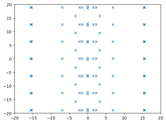
import matplotlib.pyplot as plt
fig, ax = plt.subplots()
ax.set_xlim(-20,20)
ax.set_ylim(-20,20)
plt.plot([l.real for l in lams],[l.imag for l in lams],'x')
plt.show()
Experiments with reduced basis:
[13]:
# help (Q)
Qred = MultiVector(Q[0], 0)

for fs in np.linspace(0,0.8,5):
    omega.Set(2*math.pi*fs)
    print ("fs =", fs)
    a.Assemble()

    inv = a.mat.Inverse(freedofs=fes.FreeDofs(), inverse="sparsecholesky")
    M1 = -inv@b.mat
    M2 = -inv@c.mat
    Q = SOAR(M1,M2, nr_eigs)
    lams, vecs = SolveProjected(a.mat, b.mat, c.mat, Q)
    Z = (Q * vecs).Evaluate()
    for vec in Z: vec /= Norm(vec)

    for lam, vec in zip(lams, Z):
      if abs(lam) < 6:
        if lam.imag > 1e-8:
            hvr = vec.CreateVector()
            hvi = vec.CreateVector()
            for i in range(len(vec)):
                hvr[i] = vec[i].real
                hvi[i] = vec[i].imag
            Qred.Append (hvr)
            Qred.Append (hvi)
        if abs(lam.imag) < 1e-8:
            hvr = vec.CreateVector()
            for i in range(len(vec)):
                hvr[i] = vec[i].real
            Qred.Append (hvr)

Qred.Orthogonalize()
lamsred, vecsred = SolveProjected(a.mat, b.mat, c.mat, Qred)

print ("dim Qred=", len(Qred))
fs = 0.0
fs = 0.2
fs = 0.4
fs = 0.6000000000000001
fs = 0.8
dim Qred= 40
[14]:
fs = []
ks =[]
ksi =[]

A1m = InnerProduct(Qred, a1.mat*Qred, conjugate = True)
A2m = InnerProduct(Qred, a2.mat*Qred, conjugate = True)
Bm = InnerProduct(Qred, b.mat*Qred, conjugate = True)
Cm = InnerProduct(Qred, c.mat*Qred, conjugate = True)

for fi in np.linspace(0, 0.7, 1000):
    # print ("fi =", fi)
    omega.Set(2*math.pi*fi)
    Am = A1m - omega.Get()**2 * A2m
    lamsred, vecsred = SolveProjectedSmall(Am, Bm, Cm)

    for lamred in lamsred:
        if abs(lamred.real) < 2 and lamred.imag >= 0 and lamred.imag < 6.29:
            fs.append(fi)
            ks.append(lamred.imag)
            ksi.append(lamred.real)
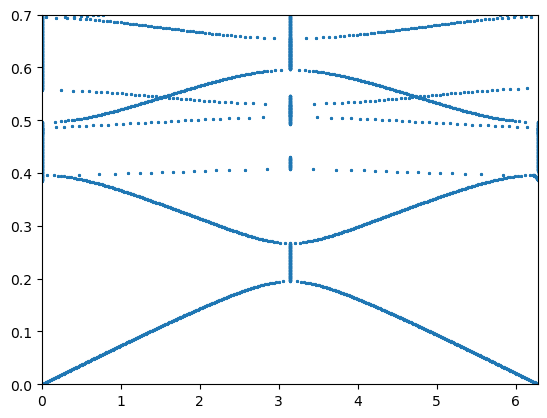
Agrees very well with Scheiber et al, path \(\Gamma-X\):
[15]:
fig, ax = plt.subplots()
ax.set_xlim(0,6.28)
ax.set_ylim(0,0.7)
plt.plot(ks, fs, "*", ms=2)
plt.show()
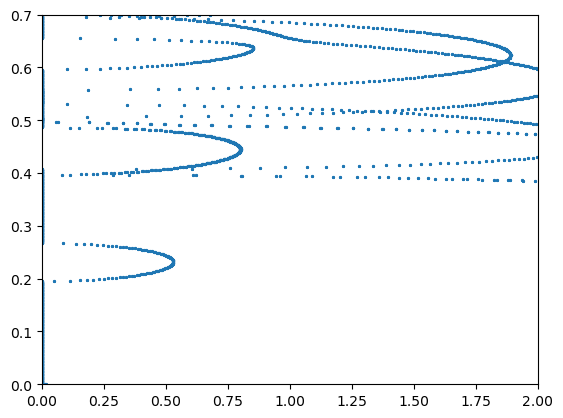
[16]:
fig, ax = plt.subplots()
ax.set_xlim(0,2)
ax.set_ylim(0,0.7)
plt.plot(ksi, fs, "*", ms=2)
plt.show()
[17]:
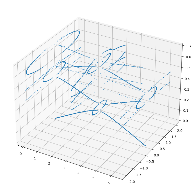
from mpl_toolkits.mplot3d import Axes3D
fig = plt.figure(figsize=(10,10))
ax = fig.add_subplot(111, projection='3d')
ax.set_zlim(0,0.7)
plt.plot(ks, ksi, fs, "*", ms=1)
plt.show()
[ ]:
[ ]: