Adaptive mesh refinement
We are solving a stationary heat equation with highly varying coefficients. This example shows how to
model a 2D geometry be means of line segments
apply a Zienkiewicz-Zhu type error estimator. The flux is interpolated into an H(div)-conforming finite element space.
loop over several refinement levels
Download: adaptive.py
from ngsolve import *
from netgen.geom2d import SplineGeometry


#   point numbers 0, 1, ... 11
#   sub-domain numbers (1), (2), (3)
#
#
#             7-------------6
#             |             |
#             |     (2)     |
#             |             |
#      3------4-------------5------2
#      |                           |
#      |             11            |
#      |           /   \           |
#      |         10 (3) 9          |
#      |           \   /     (1)   |
#      |             8             |
#      |                           |
#      0---------------------------1
#

def MakeGeometry():
    geometry = SplineGeometry()

    # point coordinates ...
    pnts = [ (0,0), (1,0), (1,0.6), (0,0.6), \
             (0.2,0.6), (0.8,0.6), (0.8,0.8), (0.2,0.8), \
             (0.5,0.15), (0.65,0.3), (0.5,0.45), (0.35,0.3) ]
    pnums = [geometry.AppendPoint(*p) for p in pnts]

    # start-point, end-point, boundary-condition, domain on left side, domain on right side:
    lines = [ (0,1,1,1,0), (1,2,2,1,0), (2,5,2,1,0), (5,4,2,1,2), (4,3,2,1,0), (3,0,2,1,0), \
              (5,6,2,2,0), (6,7,2,2,0), (7,4,2,2,0), \
              (8,9,2,3,1), (9,10,2,3,1), (10,11,2,3,1), (11,8,2,3,1) ]

    for p1,p2,bc,left,right in lines:
        geometry.Append( ["line", pnums[p1], pnums[p2]], bc=bc, leftdomain=left, rightdomain=right)
    return geometry


mesh = Mesh(MakeGeometry().GenerateMesh (maxh=0.2))


fes = H1(mesh, order=3, dirichlet=[1], autoupdate=True)
u = fes.TrialFunction()
v = fes.TestFunction()

# one heat conductivity coefficient per sub-domain
lam = CoefficientFunction([1, 1000, 10])
a = BilinearForm(fes, symmetric=False)
a += lam*grad(u)*grad(v)*dx


# heat-source in sub-domain 3
f = LinearForm(fes)
f += CoefficientFunction([0, 0, 1])*v*dx

c = MultiGridPreconditioner(a, inverse = "sparsecholesky")

gfu = GridFunction(fes, autoupdate=True)
Draw (gfu)

# finite element space and gridfunction to represent
# the heatflux:
space_flux = HDiv(mesh, order=2, autoupdate=True)
gf_flux = GridFunction(space_flux, "flux", autoupdate=True)

def SolveBVP():
    a.Assemble()
    f.Assemble()
    inv = CGSolver(a.mat, c.mat)
    gfu.vec.data = inv * f.vec
    Redraw (blocking=True)


l = []

def CalcError():
    flux = lam * grad(gfu)
    # interpolate finite element flux into H(div) space:
    gf_flux.Set (flux)

    # Gradient-recovery error estimator
    err = 1/lam*(flux-gf_flux)*(flux-gf_flux)
    elerr = Integrate (err, mesh, VOL, element_wise=True)

    maxerr = max(elerr)
    l.append ( (fes.ndof, sqrt(sum(elerr)) ))
    print ("maxerr = ", maxerr)

    for el in mesh.Elements():
        mesh.SetRefinementFlag(el, elerr[el.nr] > 0.25*maxerr)


with TaskManager():
    while fes.ndof < 100000:
        SolveBVP()
        CalcError()
        mesh.Refine()

SolveBVP()


## import matplotlib.pyplot as plt

## plt.yscale('log')
## plt.xscale('log')
## plt.xlabel("ndof")
## plt.ylabel("H1 error-estimate")
## ndof,err = zip(*l)
## plt.plot(ndof,err, "-*")

## plt.ion()
## plt.show()

## input("<press enter to quit>")
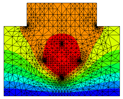
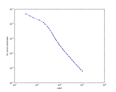
The solution on the adaptively refined mesh, and the convergence plot from matplotlib: