This page was generated from unit-3.7-opsplit/opsplit.ipynb.
3.7 DG/HDG splitting
When solving unsteady problems with an operator-splitting method it might be beneficial to consider different space discretizations for different operators.
For a problem of the form
We consider the operator splitting:
1.Step: Given \(u^0\), solve \(t^n \to t^{n+1}\): \(\quad \partial_t u + C u = 0 \Rightarrow u^{\frac12}\)
2.Step: Given \(u^{\frac12}\), solve \(t^n \to t^{n+1}\): \(\quad \partial_t u + A u = 0 \Rightarrow u^{1}\)
This splitting is only first order accurate but allows to take different time discretizations for the substeps 1 and 2.
In this example we consider the Navier-Stokes problem again (cf. unit 3.2) and want to combine
an \(H(div)\) -conforming Hybrid DG method (which is a very good discretization for Stokes-type problems) and
a standard upwind DG method for the discretization of the convection
The weak form is: Find \((\mathbf{u},p):[0,T] \to (H_{0,D}^1)^d \times L^2\), s.t.
\begin{align} \int_{\Omega} \partial_t \mathbf{u} \cdot v + \int_{\Omega} \nu \nabla \mathbf{u} \nabla \mathbf{v} + \mathbf{u} \cdot \nabla \mathbf{u} \ \mathbf{v} - \int_{\Omega} \operatorname{div}(\mathbf{v}) p &= \int f \mathbf{v} && \forall \mathbf{v} \in (H_{0,D}^1)^d, \\ - \int_{\Omega} \operatorname{div}(\mathbf{u}) q &= 0 && \forall q \in L^2, \\ \quad \mathbf{u}(t=0) & = \mathbf{u}_0 \end{align}
Again, we consider the benchmark setup from http://www.featflow.de/en/benchmarks/cfdbenchmarking/flow/dfg_benchmark2_re100.html . The geometry:
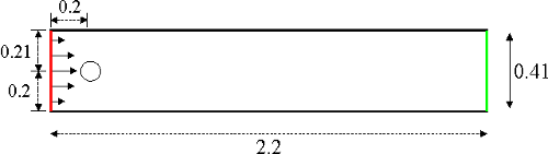
The viscosity is set to \(\nu = 10^{-3}\).
[1]:
order = 3
# import libraries, set up geometry and generate mesh
from ngsolve import *
from ngsolve.webgui import Draw
from netgen.occ import *
shape = Rectangle(2,0.41).Circle(0.2,0.2,0.05).Reverse().Face()
shape.edges.name="cyl"
shape.edges.Min(X).name="inlet"
shape.edges.Max(X).name="outlet"
shape.edges.Min(Y).name="wall"
shape.edges.Max(Y).name="wall"
mesh = Mesh(OCCGeometry(shape, dim=2).GenerateMesh(maxh=0.07)).Curve(order)
For the HDG formulation we use the product space with
\(BDM_k\): \(H(div)\) conforming FE space (degree k)
Vector facet space: facet functions of degree k (vector valued and only in tangential direction)
piecewise polynomials up to degree \(k-1\) for the pressure
HDG spaces
[2]:
V1 = HDiv ( mesh, order = order, dirichlet = "wall|cyl|inlet" )
V2 = TangentialFacetFESpace(mesh, order = order, dirichlet = "wall|cyl|inlet" )
Q = L2( mesh, order = order-1)
V = FESpace ([V1,V2,Q])

u, uhat, p = V.TrialFunction()
v, vhat, q = V.TestFunction()
Parameter and directions (normal / tangential projection):
[3]:
nu = 0.001 # viscosity
n = specialcf.normal(mesh.dim)
h = specialcf.mesh_size
def tang(vec):
    return vec - (vec*n)*n
Stokes discretization
The bilinear form to the HDG (see unit-2.8-DG for scalar HDG) discretized Stokes problem is:
\begin{align*} K_h((\mathbf{u}_T,\mathbf{u}_F,p),(\mathbf{v}_T,\mathbf{v}_F,q) := & \displaystyle \sum_{T\in\mathcal{T}} \left\{ \int_{T} \nu {\nabla} {\mathbf{u}_T} \! : \! {\nabla} {\mathbf{v}_T} \ d {x} - \int_{\Omega} \operatorname{div}(\mathbf{u}) q \ d {x} - \int_{\Omega} \operatorname{div}(\mathbf{v}) p \ d {x} \right. \\ & \qquad \left. - \int_{\partial T} \nu \frac{\partial {\mathbf{u}_T}}{\partial {n} } [ \mathbf{v} ]_t \ d {s} - \int_{\partial T} \nu \frac{\partial {\mathbf{v}_T}}{\partial {n} } [ \mathbf{u} ]_t \ d {s} + \int_{\partial T} \nu \frac{\alpha k^2}{h} [\mathbf{u}]_t [\mathbf{v}]_t \ d {s} \right\} \end{align*}
where \([\cdot]_t\) is the tangential projection of the jump \((\cdot)_T - (\cdot)_F\).
[4]:
alpha = 4  # SIP parameter
dS = dx(element_boundary=True)
a = BilinearForm ( V, symmetric=True)
a += nu * InnerProduct ( Grad(u), Grad(v) ) * dx
a += nu * InnerProduct ( Grad(u)*n, tang(vhat-v) ) * dS
a += nu * InnerProduct ( Grad(v)*n, tang(uhat-u) ) * dS
a += nu * alpha*order*order/h * InnerProduct(tang(vhat-v), tang(uhat-u)) * dS
a += (-div(u)*q - div(v)*p) * dx
a.Assemble()
[4]:
<ngsolve.comp.BilinearForm at 0x7efe4c4f5d70>
The mass matrix is simply
\begin{align*} M_h((\mathbf{u}_T,\mathbf{u}_F,p),(\mathbf{v}_T,\mathbf{v}_F,q) := \int_{\Omega} \mathbf{u}_T \cdot \mathbf{v}_T dx \end{align*}
[5]:
m = BilinearForm(u * v * dx, symmetric=True).Assemble()
Initial conditions
As initial condition we solve the Stokes problem:
[6]:
gfu = GridFunction(V)

U0 = 1.5
uin = CF( (U0*4*y*(0.41-y)/(0.41*0.41),0) )
gfu.components[0].Set(uin, definedon=mesh.Boundaries("inlet"))

invstokes = a.mat.Inverse(V.FreeDofs(), inverse="umfpack")
gfu.vec.data += invstokes @ -a.mat * gfu.vec
[7]:
scenes = [ \
    Draw( gfu.components[0], mesh, "velocity"), \
    Draw( gfu.components[2], mesh, "pressure")];
Application of convection
In the operator splitted approach we want to apply only operator applications for the convection part. Further, we want to do this in a usual DG setting. As a model problem we use the following procedure:
Given \((\mathbf{u},p)\) in HDG space: project into \(\hat{\mathbf{u}}\) in usual DG space
Solve \(\partial_t \hat{\mathbf{u}} = C \hat{\mathbf{u}}\) by explicit scheme (involves convection evaluations and mass matrix operations only)
Solve Unsteady Stokes step with r.h.s. from convection sub-problem. To this end evaluate mixed mass matrix \(\int \hat{\mathbf{u}} \cdot \mathbf{v}\) to obtain a functional on the HDG space
For the projection steps we use mixed mass matrices:
\(M_m\) : \(HDG \times DG \to \mathbb{R}\)
\(M_m^T\) : \(DG \times HDG \to \mathbb{R}\)
\(M_{DG}\) : \(DG \times DG \to \mathbb{R}\) (block diagonal)
To set up mixed mass matrices we use a bilinear form with two different FESpaces.
We do not assemble the matrices as we will only need the matrix-vector applications of \(M_m\), \(M_m^T\) and \(M_{DG}^{-1}\).
There is a more elegant version (ConvertL2Operator, similar to TraceOperator) that we discuss below.
mixed mass matrices
[8]:
VL2 = VectorL2(mesh, order=order, piola=True)
uL2, vL2 = VL2.TnT()
bfmixed = BilinearForm ( vL2*u*dx, nonassemble=True )
bfmixedT = BilinearForm ( uL2*v*dx, nonassemble=True)
convection operator
convection operation with standard Upwinding
No set up of the matrix (only interested in operator applications)
for the advection velocity we use the \(H(div)\)-conforming velocity (which is pointwise divergence free).
[9]:
vel = gfu.components[0]
convL2 = BilinearForm( (-InnerProduct(Grad(vL2) * vel, uL2)) * dx, nonassemble=True )
un = InnerProduct(vel,n)
upwindL2 = IfPos(un, un*uL2, un*uL2.Other(bnd=uin))

dskel_inner  = dx(skeleton=True)
dskel_bound  = ds(skeleton=True)

convL2 += InnerProduct (upwindL2, vL2-vL2.Other()) * dskel_inner
convL2 += InnerProduct (upwindL2, vL2) * dskel_bound
Solution of convection steps as an operator (BaseMatrix)
We now define the solution of the convection problem for an initial data \(u\) in the HDG space. The return value (y) is \(M_m \hat{u}\) where \(\hat{u}\) is the solution of several explicit Euler steps of the convection problem
[10]:
class PropagateConvection(BaseMatrix):
    def __init__(self,tau,steps):
        super(PropagateConvection, self).__init__()
        self.tau = tau; self.steps = steps
        self.h = V.ndof; self.w = V.ndof # operator domain and range
        self.mL2 = VL2.Mass(Id(mesh.dim)); self.invmL2 = self.mL2.Inverse()
        self.vecL2 = bfmixed.mat.CreateColVector() # temp vector
    def Mult(self, x, y):
        self.vecL2.data = self.invmL2 @ bfmixed.mat * x # <- project from Hdiv to L2
        for i in range(self.steps):
            self.vecL2.data -= self.tau/self.steps * self.invmL2 @ convL2.mat * self.vecL2
        y.data = bfmixedT.mat * self.vecL2
    def CreateColVector(self):
        return CreateVVector(self.h)
The operator splitted method (Yanenko splitting)
Setup of \(M^*\):
[11]:
t = 0; tend = 0
tau = 0.01; substeps = 10

mstar = m.mat.CreateMatrix()
mstar.AsVector().data = m.mat.AsVector() + tau * a.mat.AsVector()
inv = mstar.Inverse(V.FreeDofs(), inverse="umfpack")
The time loop:
[12]:
for s in scenes : s.Draw()
[13]:
%%time
tend += 1
res = gfu.vec.CreateVector()
convpropagator = PropagateConvection(tau,substeps)
while t < tend:
    gfu.vec.data += inv @ (convpropagator - mstar) * gfu.vec
    t += tau
    print ("\r  t =", t, end="")
    for s in scenes : s.Redraw()
  t = 1.0000000000000007CPU times: user 8.34 s, sys: 20.3 ms, total: 8.36 s
Wall time: 8.34 s
ConvertL2Operator
Instead of doing the conversion between the spaces "by hand", we can use the convenience operator ConvertL2Operator that realizes $ M_{DG}^{-1} :nbsphinx-math:`cdot `M_m $:
[14]:
HDG_to_L2 = V1.ConvertL2Operator(VL2) @ Embedding(V.ndof, V.Range(0)).T
The transpose of \(M_{DG}^{-1} \cdot M_m\) is \(M_m^T \cdot M_{DG}^{-1}\)
V1.ConvertL2Operator(VL2): V1 \(\to\) VL2V1.ConvertL2Operator(VL2).T: VL2' \(\to\) V1'
Overwrite the application and use the ConvertL2Operator instead ot the mixed mass matrices:
[15]:
def NewMult(self, x, y):
    self.vecL2.data = HDG_to_L2 * x # <- project from Hdiv to L2
    for i in range(self.steps):
        self.vecL2.data -= tau/self.steps*self.invmL2@convL2.mat*self.vecL2
    y.data = HDG_to_L2.T @ self.mL2 * self.vecL2

PropagateConvection.Mult = NewMult
The time loop:
[16]:
for s in scenes : s.Draw()
[17]:
%%time
tend += 1
convpropagator = PropagateConvection(tau,substeps)
while t < tend:
    gfu.vec.data += inv @ (convpropagator - mstar) * gfu.vec
    t += tau
    print ("\r  t =", t, end="")
    for s in scenes : s.Redraw()
  t = 2.0000000000000013CPU times: user 8.04 s, sys: 48.7 ms, total: 8.09 s
Wall time: 8.05 s
Tasks:
Implement higher order Splitting (e.g. Strang) schemes
Implement IMEX schemes and compare