This page was generated from unit-3.8-simplehyp/shallow2D.ipynb.

3.8 A Nonlinear conservation law: shallow water equation in 2D

We consider the shallow water equations as an example of a nonlinear conservation law, i.e. we consider

\[\partial_t \mathbf{U} + \operatorname{div}(\mathbf{F} (\mathbf{U} )) = 0 \qquad in \qquad \Omega \times[0,T],\]

with

\[\mathbf{U} = (h, \mathbf{w}) = (h, hu, hv) = (\mathbf{u}_1, \mathbf{u}_2, \mathbf{u}_3)\]

and

\[\begin{split}\mathbf{F}(\mathbf{U}) = \left( \begin{array}{c@{}c@{\qquad}c@{}c} h u & & h v & \\ h u^2 &+ \frac12 g h^2 & h u v & \\ h u v & & h v^2 & + \frac12 g h^2 \end{array} \right) = \left( \begin{array}{cc} \mathbf{u}_2 & \mathbf{u}_3 \\ \frac{\mathbf{u}_2^2}{\mathbf{u}_1} + \frac12 g \mathbf{u}_1^2 & \frac{\mathbf{u}_2 \mathbf{u}_3}{\mathbf{u}_1} \\ \frac{\mathbf{u}_2 \mathbf{u}_3}{\mathbf{u}_1} & \frac{\mathbf{u}_3^2}{\mathbf{u}_1} + \frac12 g \mathbf{u}_1^2 \end{array} \right) = \left( \begin{array}{cc} h \mathbf{w}^T \\ h \mathbf{w} \otimes \mathbf{w} + \frac12 g h^2 \mathbf{I} \end{array} \right)\end{split}\]

Jacobian of the flux for shallow water:

\begin{align*} \mathbf{A}_1 & = \left(\begin{array}{ccc} 0 & 1 & 0 \\ - \frac{\mathbf{u}_2^2}{\mathbf{u}_1^2} + g \mathbf{u}_1 & 2 \frac{\mathbf{u}_2}{\mathbf{u}_1} & 0 \\ - \frac{\mathbf{u}_2 \mathbf{u}_3}{\mathbf{u}_1^2} & \frac{\mathbf{u}_3}{\mathbf{u}_1} & \frac{\mathbf{u}_2}{\mathbf{u}_1} \end{array} \right) = \left( \begin{array}{ccc} 0 & 1 & 0 \\ - u^2 + g h & 2 u & 0 \\ - u v & v & u \end{array} \right) \end{align*}

\begin{align*} \mathbf{A}_2 & = \left( \begin{array}{ccc} 0 & 0 & 1 \\ - \frac{\mathbf{u}_2\mathbf{u}_3}{\mathbf{u}_1^2} & \frac{\mathbf{u}_3}{\mathbf{u}_1} & \frac{\mathbf{u}_2}{\mathbf{u}_1} \\ - \frac{\mathbf{u}_3^2}{\mathbf{u}_1^2} + g \mathbf{u}_1 & 0 & 2\frac{\mathbf{u}_3}{\mathbf{u}_1} \end{array} \right) = \left( \begin{array}{ccc} 0 & 0 & 1 \\ - uv & v & u \\ - v^2 + gh & 0 & 2 v \end{array} \right) \end{align*}

\begin{align*} \mathbf{A}(\mathbf{u}, \mathbf{n}) & = n_1 \mathbf{A}_1 + n_2 \mathbf{A}_2 = \left( \begin{array}{ccc} 0 & n_1 & n_2 \\ - u \alpha - g h n_1 & \alpha + u n_1 & u n_2 \\ - v \alpha - g h n_2 & v n_1 & \alpha + v n_2 \end{array} \right), \quad \text{ with } \alpha = (\mathbf{u}, \mathbf{n}), \end{align*}

\[\text{spectrum:} \qquad \rho( \mathbf{A}(\mathbf{u}, \mathbf{n}) ) = \{ \alpha + \sqrt{g h}, \alpha, \alpha - \sqrt{g h} \}\]

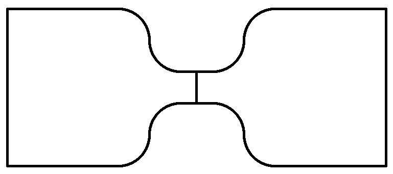
The dam break problem (geometry)

# geometry description (including boundary/mat names)
from ngsolve import *
from netgen.occ import *
from ngsolve.webgui import *
wp = WorkPlane()
wp.MoveTo(-12,-5).LineTo(-3,-5).NameVertex("fillet")
wp.LineTo(-3,-1).NameVertex("fillet")
wp.LineTo(0,-1).LineTo(0,0).LineTo(-12,0).Close()
geo = wp.Face()
geo = geo.MakeFillet(list(set(geo.vertices["fillet"])),2)
geo = geo + geo.Mirror(Axis((0,0,0),X)).Reversed()
geo = Glue([geo,geo.Mirror(Axis((0,0,0),Y)).Reversed()])
geo.faces.Min(X).name="upperlevel"
geo.faces.Max(X).name="lowerlevel"
geo.edges.name = "wall"
geo.edges.Nearest((0,0)).name = "dam"
#Draw(geo)
geo = OCCGeometry(geo,dim=2)

from ngsolve import *
from ngsolve.webgui import Draw
mesh = Mesh(geo.GenerateMesh(maxh=2))
mesh.Curve(3)
Draw(mesh)

BaseWebGuiScene

Vectorial (dim=3) approximation space:

order = 2
fes = L2(mesh,order=order)**3
#fes = L2(mesh,order=order,dim=3)

initial and boundary conditions

U,V = fes.TnT() # "Trial" and "Test" function
h, hu, hv = U

# initial conditions
h0mat = {"upperlevel" : 10, "lowerlevel" : 2}
U0 = CF((mesh.MaterialCF(h0mat),0,0))

# boundary conditions
hbndreg = mesh.BoundaryCF({"wall" : h, "dam" : 0})
hubndreg = mesh.BoundaryCF({"wall" : -hu, "dam" : 0})
hvbndreg = mesh.BoundaryCF({"wall" : -hv, "dam" : 0})

Ubnd = CF((hbndreg,hubndreg,hvbndreg))

# constant for gravitational force
g=1

Flux definition and numerical flux choice (Lax-Friedrich)

\[\begin{split}\mathbf{F}(\mathbf{U}) = \left( \begin{array}{c@{}c@{\qquad}c@{}c} h u & & h v & \\ h u^2 &+ \frac12 g h^2 & h u v & \\ h u v & & h v^2 & + \frac12 g h^2 \end{array} \right) = \left( \begin{array}{cc} \mathbf{u}_2 & \mathbf{u}_3 \\ \frac{\mathbf{u}_2^2}{\mathbf{u}_1} + \frac12 g \mathbf{u}_1^2 & \frac{\mathbf{u}_2 \mathbf{u}_3}{\mathbf{u}_1} \\ \frac{\mathbf{u}_2 \mathbf{u}_3}{\mathbf{u}_1} & \frac{\mathbf{u}_3^2}{\mathbf{u}_1} + \frac12 g \mathbf{u}_1^2 \end{array} \right) = \left( \begin{array}{cc} h \mathbf{w}^T \\ h \mathbf{w} \otimes \mathbf{w} + \frac12 g h^2 \mathbf{I} \end{array} \right)\end{split}\]

def F(U):
    h, hvx, hvy = U
    vx = hvx/h
    vy = hvy/h
    return CF(((hvx,hvy),
               (hvx*vx + 0.5*g*h**2, hvx*vy),
               (hvx*vy, hvy*vy + 0.5*g*h**2)),dims=(3,2))

\[\hat{\mathbf{F}}(\mathbf{U}) \cdot \mathbf{n} = \frac{(\mathbf{F}(\mathbf{U}^l)+\mathbf{F}(\mathbf{U}^r)}{2} \cdot \mathbf{n} + \frac{|\lambda|}{2} (\mathbf{U}^l - \mathbf{U}^r), \quad (\cdot^l: \text{current element}, \quad \cdot^r: \text{neighbor element})\]

n = specialcf.normal(mesh.dim)
def Max(u,v):
    return IfPos(u-v,u,v)
def Fmax(A,B): # max. characteristic speed:
    ha, hua, hva = A
    hb, hub, hvb = B
    vnorma = sqrt(hua**2+hva**2)/ha
    vnormb = sqrt(hub**2+hvb**2)/hb
    return Max(vnorma+sqrt(g*A[0]),vnormb+sqrt(g*B[0]))

def Fhatn(U): # numerical flux
    Uhat = U.Other(bnd=Ubnd)
    return (0.5*F(U)+0.5*F(Uhat))*n + Fmax(U,Uhat)/2*(U-Uhat)

DG formulation

We recall that a BilinearForm is allowed to be nonlinear in the first argument.

def DGBilinearForm(fes,F,Fhatn,Ubnd):
    a = BilinearForm(fes, nonassemble=True)
    a += - InnerProduct(F(U),Grad(V)) * dx
    a += InnerProduct(Fhatn(U),V) * dx(element_boundary=True)
    return a

a = DGBilinearForm(fes,F,Fhatn,Ubnd)

Simple fix to deal with shocks: artificial diffusion:

from DGdiffusion import AddArtificialDiffusion

artvisc = Parameter(1.0)
if order > 0:
    AddArtificialDiffusion(a,Ubnd,artvisc,compile=True)

Visualization of solution quantities

gfu = GridFunction(fes)
gfh, gfhu, gfhv = gfu
gfvu = gfhu/gfh
gfvv = gfhv/gfh
momentum = CF((gfhu,gfhv))
velocity = CF((gfvu,gfvv))
gfu.Set(U0)
scenes = [ \
    Draw(momentum,mesh,"mom"),
    Draw(velocity,mesh,"vel"),
    Draw(gfh,mesh,"h") ]

Explicit Euler time stepping

def TimeLoop(a,gfu,dt,T,nsamplings=100,scenes=scenes,multidim_draw=False,md_nsamplings=20):
    if multidim_draw:
        gfu_t = GridFunction(gfu.space,multidim=True)
    #gfu.Set(U0)
    res = gfu.vec.CreateVector()
    fes = a.space
    t = 0; i = 0
    nsteps = int(ceil(T/dt))
    invma = fes.Mass(1).Inverse() @ a.mat
    if multidim_draw:
        gfu_t.AddMultiDimComponent(gfu.vec)
    with TaskManager():
        while t <= T - 0.5*dt:
            res = invma * gfu.vec
            gfu.vec.data -= dt * res
            t += dt
            if (i+1) % int(nsteps/nsamplings) == 0:
                for s in scenes: s.Redraw()
            if multidim_draw and (i+1) % int(nsteps/md_nsamplings) == 0:
                gfu_t.AddMultiDimComponent(gfu.vec)
            i+=1
            print("\rt = {:.10}".format(t),end="")
    for s in scenes: s.Redraw()
    if multidim_draw:
        return gfu_t

gfu.Set(U0)
with TaskManager():
    gfu_t = TimeLoop(a,gfu,dt=0.0025,T=15,multidim_draw=True,md_nsamplings=5)

t = 15.0

Draw(gfu_t.components[0],mesh,"h",interpolate_multidim=True,animate=True,
     deformation=True, settings = {"camera" :
                                   {"transformations" :
                                    [{ "type": "rotateX", "angle": -20},
                                     { "type": "rotateZ", "angle": 0}]}},
     min=2, max=5, autoscale=False)

BaseWebGuiScene

Tasks

You may play around with this example.

• change the artificial diffusion parameter: How does it influence the solution

• change boundary conditions: left boundary -> fixed height and non-reflecting

• change the initial heights

• introduce a (circular) obstacle below the dam

• Generate output to create a video: To this end take a look at the final unit of this section.