This page was generated from unit-3.2-navierstokes/navierstokes.ipynb.

3.2 Incompressible Navier-Stokes equations

As in the whetting the appetite demo we consider the unsteady Navier Stokes equations

Find \((u,p):[0,T] \to (H_{0,D}^1)^d \times L^2\), s.t.

\begin{align*} \int_{\Omega} \partial_t u \cdot v + \int_{\Omega} \nu \nabla u \nabla v + u \cdot \nabla u v - \int_{\Omega} \operatorname{div}(v) p &= \int f v && \forall v \in (H_{0,D}^1)^d, \\ - \int_{\Omega} \operatorname{div}(u) q &= 0 && \forall q \in L^2, \\ \quad u(t=0) & = u_0 \end{align*}

Schäfer-Turek benchmark

We consider the benchmark setup of from http://www.featflow.de/en/benchmarks/cfdbenchmarking/flow/dfg_benchmark2_re100.html . The geometry is a 2D channel with a circular obstacle which is positioned (only slightly) off the center of the channel. The geometry:

The viscosity is set to \(\nu = 10^{-3}\).

# import libarries, define geometry and generate mesh
from ngsolve import *
from ngsolve.webgui import Draw
from netgen.occ import *
from netgen.webgui import Draw as DrawGeo
shape = Rectangle(2,0.41).Circle(0.2,0.2,0.05).Reverse().Face()
shape.edges.name="cyl"
shape.edges.Min(X).name="inlet"
shape.edges.Max(X).name="outlet"
shape.edges.Min(Y).name="wall"
shape.edges.Max(Y).name="wall"
mesh = Mesh(OCCGeometry(shape, dim=2).GenerateMesh(maxh=0.07)).Curve(3)

DrawGeo (shape)
Draw (mesh)

BaseWebGuiScene

Viscosity:

# viscosity
nu = 0.001

Taylor-Hood velocity-pressure pair

We use a Taylor-Hood discretization of degree \(k\). The finite element space for the (vectorial) velocity \(\mathbf{u}\) and the pressure \(p\) are:

\begin{align} \mathbf{u} \in \mathbf{V} &= \{ v \in H^1(\Omega) | v|_T \in \mathcal{P}^k(T) \}^2 \\ p \in Q &= \{ q \in H^1(\Omega) | q|_T \in \mathcal{P}^{k-1}(T) \} \end{align}

k = 3
V = VectorH1(mesh,order=k, dirichlet="wall|cyl|inlet")
Q = H1(mesh,order=k-1)
X = V*Q

The VectorH1 is the product space of two H1 spaces with convenience operators for identity, grad(Grad) and div.

Stokes problem for initial values

Find \(\mathbf{u} \in \mathbf{V}\), \(p \in Q\) so that

\begin{align} \int_{\Omega} \nu \nabla \mathbf{u} : \nabla \mathbf{v} - \int_{\Omega} \operatorname{div}(\mathbf{v}) p &= \int \mathbf{f} \cdot \mathbf{v} && \forall \mathbf{v} \in \mathbf{V}, \\- \int_{\Omega} \operatorname{div}(\mathbf{u}) q &= 0 && \forall q \in Q, \end{align}

with boundary conditions:

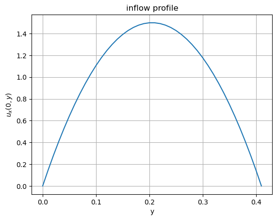
• the inflow boundary data ('inlet') with mean value \(1\)

\begin{align} u_x(0,y) &= 6 y(0.41-y)/(0.41)^2, \quad \int_{0}^{0.41} u_x(0,y) dy = 1 \\ u_y(0,y) &= 0 \end{align}

• "do-nothing" boundary conditions on the ouflow ('outlet') and

• homogeneous Dirichlet conditions on all other boundaries ('wall').

gfu = GridFunction(X)
velocity, pressure = gfu.components
# parabolic inflow at bc=1:
uin = CoefficientFunction((1.5*4*y*(0.41-y)/(0.41*0.41),0))
velocity.Set(uin, definedon=mesh.Boundaries("inlet"))

Draw(velocity,mesh,"u")
Draw(pressure,mesh,"p")

BaseWebGuiScene

inflow profile plot:

import matplotlib; import numpy as np; import matplotlib.pyplot as plt;
%matplotlib inline
s = np.arange(0.0, 0.42, 0.01)
bvs = 6*s*(0.41-s)/(0.41)**2
plt.plot(s, bvs)
plt.xlabel('y'); plt.ylabel('$u_x(0,y)$'); plt.title('inflow profile')
plt.grid(True)
plt.show()

To solve the Stokes (and later the Navier-Stokes) problem, we introduce the bilinear form:

\[a((u,p),(v,q)) := \int_{\Omega} \nu \nabla u : \nabla v - \operatorname{div}(v) p - \operatorname{div}(u) q\]

and directly use it to solve the Stokes problem for suitable initial values:

(u,p), (v,q) = X.TnT()

a = BilinearForm(X)
stokes = (nu*InnerProduct(grad(u),grad(v))-div(u)*q-div(v)*p)*dx
a += stokes
a.Assemble()

f = LinearForm(X)
f.Assemble()

res = f.vec - a.mat*gfu.vec
inv_stokes = a.mat.Inverse(X.FreeDofs())
gfu.vec.data += inv_stokes * res

sceneu = Draw(velocity,mesh,"u")
scenep = Draw(pressure,mesh,"p")

IMEX time discretization

For the time integration we consider an semi-implicit Euler method (IMEX) where the convection is treated only explicitly and the remaining part implicitly:

Find \((\mathbf{u}^{n+1},p^{n+1}) \in X = \mathbf{V} \times Q\), s.t. for all \((\mathbf{v},q) \in X = \mathbf{V} \times Q\)

\begin{align} \underbrace{m(\mathbf{u}^{n+1},\mathbf{v}) + \Delta t ~\cdot~a((\mathbf{u}^{n+1},p^{n+1}),(\mathbf{v},q))}_{ \to M^\ast} ~=~m(\mathbf{u}^{n},\mathbf{v}) - \Delta t ~\cdot~c(\mathbf{u}^{n}; \mathbf{u}^{n},\mathbf{v}) \end{align}

with \begin{align} m(\mathbf{u},\mathbf{v}) = \int \mathbf{u} \cdot \mathbf{v} \end{align}

and \begin{align} c(\mathbf{w},\mathbf{u},\mathbf{v}) = \int \mathbf{w} \cdot \nabla \mathbf{u} \cdot \mathbf{v} \end{align}

We prefer the incremental form (as it homogenizes the boundary conditions): \begin{align} m(\delta \mathbf{u}^{n+1},\mathbf{v}) + \Delta t ~\cdot~a((\delta \mathbf{u}^{n+1},\delta p^{n+1}),(\mathbf{v},q)) ~=~ \Delta t (-a((\mathbf{u}^{n},p^n),(\mathbf{v},q)) -c(\mathbf{u}^{n}; \mathbf{u}^{n},\mathbf{v})) \end{align}

dt = 0.001
# matrix for implicit part of IMEX(1) scheme:
mstar = BilinearForm(X)
mstar += InnerProduct(u,v)*dx + dt*stokes
mstar.Assemble()
inv = mstar.mat.Inverse(X.FreeDofs())

Next, we want to evaluate the convection term \(c(u^n;u^n,v)\) for given \(u^n\), i.e. a linear form. We can do this by setting up a LinearForm

fc = LinearForm(X)
fc += (Grad(gfu) * gfu) * v * dx

Then, for \(u^n =\)gfu a call fc.Assemble() yields a vector fc.vecrepresenting the linear form.

Alternatively, we can use the semi-linear form structure of the convection form and put it into a BilinearForm (which indeed is able to represent non-bilinear forms as we will discuss in more detail in unit-3.3). We will not need the assembly (or the storage of a sparse matrix) though:

conv = BilinearForm(X, nonassemble = True)
conv += (Grad(u) * u) * v * dx

Instead of assembling a LinearForm in every time step, we use an operator application of a BilinearForm, see unit-2.11 or the next units for more details.

The BilinearForm(which indeed is rather a semi-linear form) can compute the linear form at a given state u:

• either by a call conv.Apply(gfu.vec,res) where the result ends up in the vector res

• alternatively we can use the notation of an operator application conv.mat * gfu.vec yielding the same.

Below, we will use the latter.

tend = 0
gfut = GridFunction(gfu.space,multidim=0)

# implicit Euler/explicit Euler splitting method:
tend += 1
gfut.AddMultiDimComponent(gfu.vec)
t = 0; cnt = 0
while t < tend-0.5*dt:
    print ("\rt=", t, end="")

    conv.Assemble()
    res = (a.mat + conv.mat)* gfu.vec
    gfu.vec.data -= dt * inv * res

    t = t + dt; cnt += 1
    sceneu.Redraw()
    scenep.Redraw()
    if cnt % 50 == 0:
        gfut.AddMultiDimComponent(gfu.vec)

t= 0.003craete bilinearformapplication
t= 0.9990000000000008

Draw (gfut.components[0], mesh, interpolate_multidim=True, animate=True,
      min=0, max=1.9, autoscale=False, vectors = True)
Draw (gfut.components[1], mesh, interpolate_multidim=True, animate=True,
      min=-0.5, max=1, autoscale=False)

BaseWebGuiScene

In this benchmark scenario of specific interests are the forces acting on the disk (cylinder). We will discuss how to compute them next.

Supplementary 1: Computing stresses

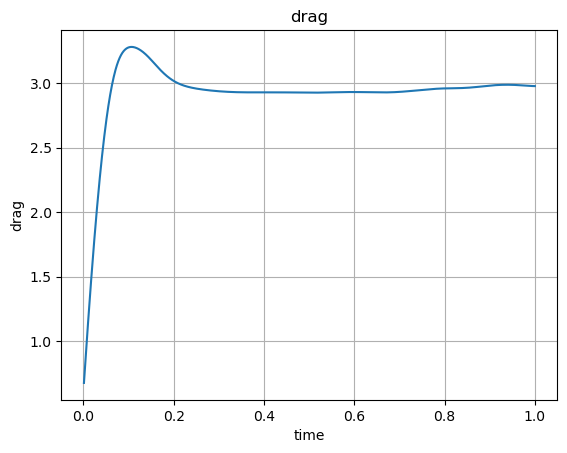
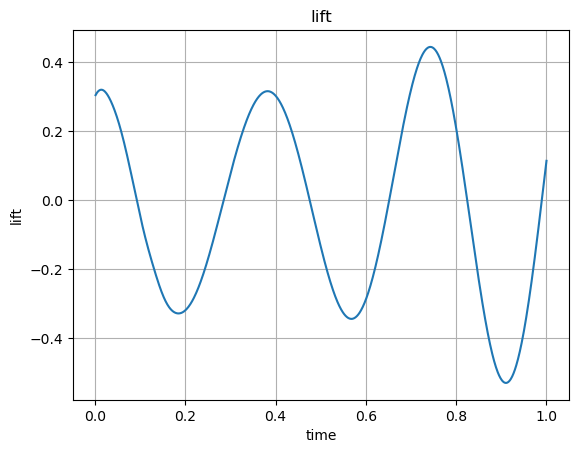
In the previously used benchmark the stresses on the obstacle are evaluated, the so-called drag and lift coefficients.

The force acting on the obstacle is

\[F_{\circ} = (F_D,F_L) = \int_{\Gamma_{cyl}} \sigma_n = \int_{\Gamma_{cyl}} (-\nu \frac{\partial u}{\partial n} + p I) \cdot n\]

The drag/lift coefficients are

\[c_D = \frac{2 }{\bar{u} L} F_D, \quad c_L = \frac{2 }{\bar{u} L} F_L.\]

where \(\bar{u} = 1\) is the mean inflow velocity and \(L = 0.41\) is the channel width.

We use the residual of our discretization to compute the forces. On the boundary degrees of freedoms of the disk we overwrote the equation by prescribing the (homogeneous) boundary conditions. The equations related to these dofs describe the force (im)balance at this boundary.

Testing the residual (functional) with the characteristic function on that boundary (in the x- or y-direction) we obtain the integrated stresses (in the x- or y-direction):

We define the functions which are characteristic functions (in terms of boundary evaluations)

drag_x_test = GridFunction(X)
drag_x_test.components[0].Set(CoefficientFunction((-20.0,0)), definedon=mesh.Boundaries("cyl"))
drag_y_test = GridFunction(X)
drag_y_test.components[0].Set(CoefficientFunction((0,-20.0)), definedon=mesh.Boundaries("cyl"))

We will collect drag and lift forces over time and therefore create empty arrays

and reset initial data (and time)

time_vals, drag_x_vals, drag_y_vals = [],[],[]

# restoring initial data
res = f.vec - a.mat*gfu.vec
gfu.vec.data += inv_stokes * res

With the same discretization as before.

Remarks: * you can call the following block several times to continue a simulation and collect more data * note that you can reset the array without rerunning the simulation

t = 0
tend = 0

tend += 1
while t < tend-0.5*dt:
    print ("\rt=", t, end="")
    res = (a.mat + conv.mat) * gfu.vec
    gfu.vec.data -= dt * inv * res
    t += dt
    time_vals.append( t )
    drag_x_vals.append(InnerProduct(res, drag_x_test.vec) )
    drag_y_vals.append(InnerProduct(res, drag_y_test.vec) )

t= 0.9990000000000008

Below you can plot the gathered drag and lift values:

# Plot drag force over time
plt.plot(time_vals, drag_x_vals)
plt.xlabel('time'); plt.ylabel('drag'); plt.title('drag'); plt.grid(True)
plt.show()

# Plot lift force over time
plt.plot(time_vals, drag_y_vals)
plt.xlabel('time'); plt.ylabel('lift'); plt.title('lift'); plt.grid(True)
plt.show()

Tasks

If you understood the tutorial so far, you may want to play around with it further. Here are some suggestions on what you could do:

• Compute drag and lift forces directly through the surface integrals and compare to the residual based evaluation

• Change the geometry and solve a driven cavity example

• Use a fully implicit time integration scheme

• Use a higher order implict or IMEX scheme for time integration