This page was generated from unit-8.7-mlset_pde/mlset_pde.ipynb.

8.7 Unfitted FEM for domains described by multiple level sets

In order to solve a partial differential equation on a stationary domain defined by multiple level set functions, we proceed similarly to the demo cutfem.ipynb, with a few key differences in order to deal with corners.

For simplicity we consider a Poisson problem on the unit square in order to show the differences between the single and multiple level set setting.

The libraries are imported as usual:

# Basic NGSolve things
from netgen.geom2d import SplineGeometry
from ngsolve import *
from ngsolve.solvers import PreconditionedRichardson as PreRic

# ngsxfem and the mlset convenience layer
from xfem import *
from xfem.mlset import *

# Visualisation
from ngsolve.webgui import *
DrawDC = MakeDiscontinuousDraw(Draw)

importing ngsxfem-2.1.2303.dev0

We want to solve the problem

\[\begin{split}\begin{aligned} -\Delta u &= f &&\text{in }\Omega\\ u &= 0 &&\text{on } \partial\Omega \end{aligned}\end{split}\]

where the domain \(\Omega\subset\widetilde\Omega\) is a subset of the meshed background domain \(\widetilde\Omega\).

geo = SplineGeometry()
geo.AddRectangle((-0.2, -0.2), (1.2, 1.2), bcs=("bottom", "right", "top", "left"))
mesh = Mesh(geo.GenerateMesh(maxh=0.1))

We define the domain as the set \(\Omega := \bigcap_i \{\phi_i < 0\}\) with \(\{\phi_i\} = \{ -y, x - 1, y - 1, -x \}\) and use a DomainTypeArray as a container for this set and to generate the boundary.

level_sets = [-y, x - 1, y - 1, -x]
level_sets_p1 = tuple(GridFunction(H1(mesh, order=1)) for i in range(len(level_sets)))
for i, lsetp1 in enumerate(level_sets_p1):
    InterpolateToP1(level_sets[i], lsetp1)
    DrawDC(lsetp1, -3.5, 2.5, mesh, "lsetp1_{}".format(i))

square = DomainTypeArray((NEG, NEG, NEG, NEG))
boundary = square.Boundary()

Finite Element spaces are defined as usual:

k = 3

V = H1(mesh, order=k, dgjumps=True)
gfu = GridFunction(V)

Multiple level set cut-information

As before, we use standard FE spaces restricted to the active part of the mesh. In order to handle multiple level sets, we need the MultiLevelsetCutInfo class:

mlci = MultiLevelsetCutInfo(mesh, level_sets_p1)

Marking the correct elements

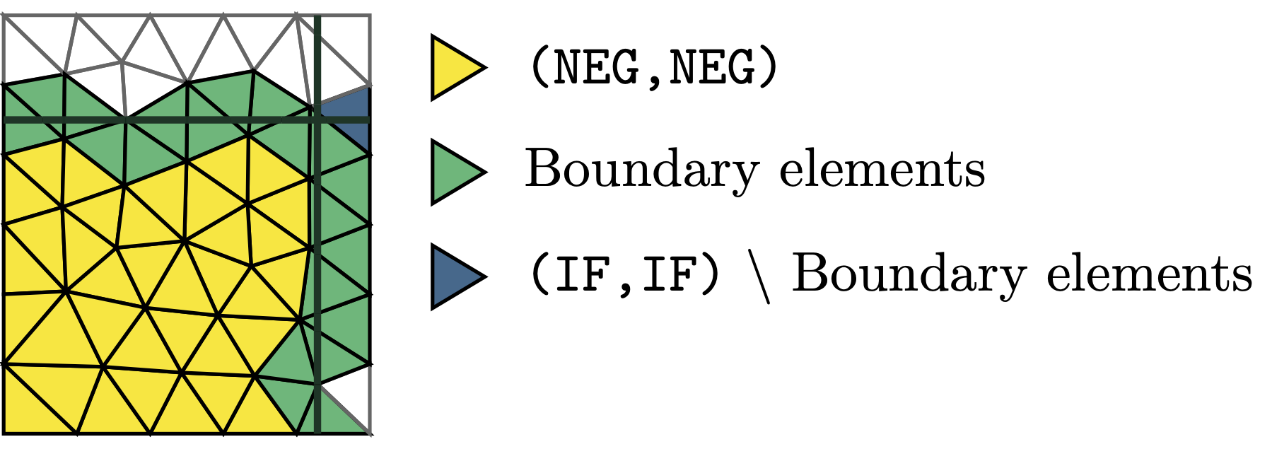
Marking the correct active elements needs to be handled differently in the multipe level set setting, since elements of the type (IF,IF) are sometimes not part of the active domain, as can be seen in the following image:

In order to select the correct active elements, the MultiLevelsetCutInfo class has a member function GetElementsWithContribution(). This takes in a tuple(ENUM), a list of such tuples or a DomainTypeArray

els_hasneg = mlci.GetElementsWithContribution(square)
els_if = mlci.GetElementsWithContribution(boundary)

Draw(BitArrayCF(els_hasneg), mesh, "els_hasneg")
Draw(BitArrayCF(els_if), mesh, "els_if")

BaseWebGuiScene

To deal with arbitraty mesh-interface cuts we use ghost-penalty stabilisation. The elements needed for this can be obtained in the same manner as before and similarly, the free degrees of freedom can also be determined as before:

facets_gp = GetFacetsWithNeighborTypes(mesh, a=els_hasneg, b=els_if,
                                       use_and=True)

freedofs = GetDofsOfElements(V, els_hasneg) & V.FreeDofs()

We implement the homogeneous Dirichlet boundary conditions using Nitsche’s trick. As each boundaty section has a different unit-normal vector, we have to decompose the Nitsche term into the different segments. Each will be added as a separate weak form, so we also require element markers for each side seperately.

Since the easient and most flexible nomenclature for each segment is the tuple of DOMAIN_TYPEs, we store these element markers in a dictionary using the tuple as the key:

els_if_single = {}
for i, dtt in enumerate(boundary):
    els_if_single[dtt] = mlci.GetElementsWithContribution(dtt)
    Draw(BitArrayCF(els_if_single[dtt]), mesh, "els_if_singe"+str(i))

Defining the weak form

As in any other unfitted problem, we define some parameters and get the trial and test functions and mesh-size coefficient functions as usual.

gamma_n = 10
gamma_s = 0.5

u, v = V.TnT()
h = specialcf.mesh_size

For the normal vectors, we use the DomainTypeArray.GetOuterNormals() functionality, see mlset_basic.ipynb

normals = square.GetOuterNormals(level_sets_p1)

We then define the cut SymbolicDifferentialSymbols for the volume, boundary and ghost-penalty facet-patch integrators, see also mlset_basic.ipynb. Note that we pass the BitArrays on which the integrators are defined to the SymbolicDiffeentialSymbol

dx = dCut(level_sets_p1, square, definedonelements=els_hasneg)
ds = {dtt: dCut(level_sets_p1, dtt, definedonelements=els_if_single[dtt])
      for dtt in boundary}
dw = dFacetPatch(definedonelements=facets_gp)

Integrators

As we have an unfitted problem, we use a RestrictedBilinearForm

a = RestrictedBilinearForm(V, element_restriction=els_hasneg, facet_restriction=facets_gp, check_unused=False)

The diffusion and ghost_penalty forms can then be added normally

a += InnerProduct(Grad(u), Grad(v)) * dx
a += gamma_s / (h**2) * (u - u.Other()) * (v - v.Other()) * dw

For the Nitsche terms, we loop over the normals dictionary. This gives us acess to both the boundary domain-tuples and the normal vectors:

for bnd, n in normals.items():
    a += -InnerProduct(Grad(u) * n, v) * ds[bnd]
    a += -InnerProduct(Grad(v) * n, u) * ds[bnd]
    a += (gamma_n * k * k / h) * InnerProduct(u, v) * ds[bnd]

We want the exact solution to be \(u = 16 x (1 - x) y (1 - y)\). To add the appropriate forcing term to the right-hand side, we do not have anything special

f = LinearForm(V)
f += 32 * (y * (1 - y) + x * (1 - x)) * v * dx

Solving the system

Now the system has been set up, we can assemble the systrem and sove in the usual manner

f.Assemble()
a.Assemble()
inv = a.mat.Inverse(freedofs=freedofs, inverse="sparsecholesky")

gfu.vec.data = PreRic(a=a, rhs=f.vec, pre=inv, freedofs=freedofs)

it = 0  ||res||_2 = 1.0491905634098577
it = 1  ||res||_2 = 9.590210798791288e-15

We can now visualise the solution:

u_ex = 16 * x * (1 - x) * y * (1 - y)
grad_u_ex = CoefficientFunction((16 * (1 - 2 * x) * y * (1 - y),
                                 16 * x * (1 - x) * (1 - 2 * y)))
DrawDC(square.Indicator(level_sets_p1), 0, gfu, mesh, "solution")

BaseWebGuiScene

And compute the error. To integrate with quadrature rules of the correct order we generate new cut SumbolicDifferentialSymbols using the .order(k) method with returns a new DifferentialSymbol which tells the Integrate to integrate with order k

err_l2 = sqrt(Integrate((gfu - u_ex)**2 * dx.order(2 * k), mesh=mesh))
err_h1 = sqrt(Integrate((Grad(gfu) - grad_u_ex)**2 * dx.order(2 * (k - 1)), mesh=mesh))
print("L2 error = {:1.3e}".format(err_l2))
print("H1 error = {:1.3e}".format(err_h1))

L2 error = 3.497e-06
H1 error = 3.809e-04