This page was generated from unit-7-optimization/01_Shape_Derivative_Levelset.ipynb.
7.1 Shape optimization via the shape derivative
In this tutorial we discuss the implementation of shape optimization algorithms to solve
The analytic solution to this problem is
This problem is solved by fixing an initial guess \(\Omega_0\subset \mathbf{R}^d\) and then considering the problem
where \(X:\mathbf{R}^d \to \mathbf{R}^d\) are (at least) Lipschitz vector fields. We approximate \(X\) by a finite element function.
Initial geometry and shape function
We choose \(f\) as
where \(\varepsilon = 0.001, a = 4/5, b = 2\). The corresponding zero level sets of this function are as follows. The green area indicates where \(f\) is negative.
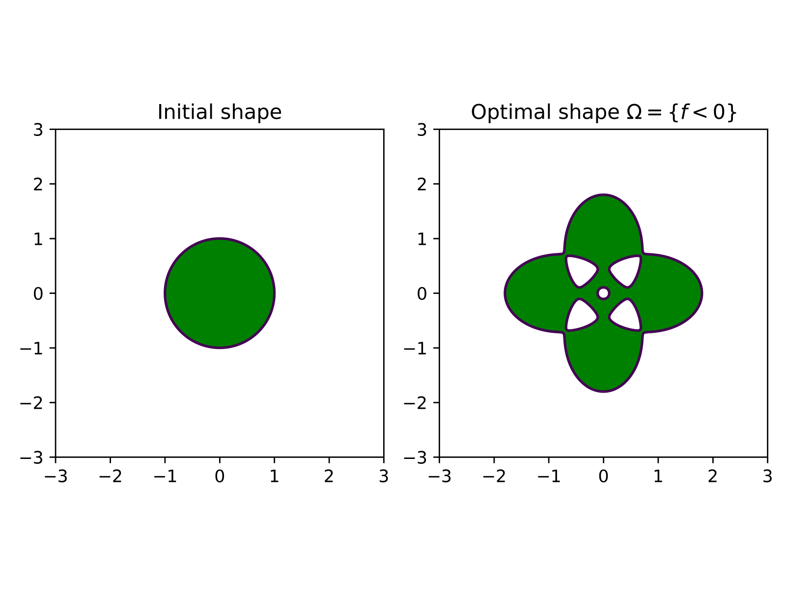
Let us set up the geometry.
[1]:
# Generate the geometry
from ngsolve import *
# load Netgen/NGSolve and start the gui
from ngsolve.webgui import Draw
from netgen.geom2d import SplineGeometry
geo = SplineGeometry()
geo.AddCircle((0,0), r = 2.5)
ngmesh = geo.GenerateMesh(maxh = 0.08)
mesh = Mesh(ngmesh)
mesh.Curve(2)
[1]:
<ngsolve.comp.Mesh at 0x7f79c305c170>
[2]:
#gfset.vec[:]=0
#gfset.Set((0.2*x,0))
#mesh.SetDeformation(gfset)
#scene = Draw(gfzero,mesh,"gfset", deformation = gfset)
[3]:
# define the function f and its gradient
a =4.0/5.0
b = 2
f = CoefficientFunction((sqrt((x - a)**2 + b * y**2) - 1) \
* (sqrt((x + a)**2 + b * y**2) - 1) \
* (sqrt(b * x**2 + (y - a)**2) - 1) \
* (sqrt(b * x**2 + (y + a)**2) - 1) - 0.001)
# gradient of f defined as vector valued coefficient function
grad_f = CoefficientFunction((f.Diff(x),f.Diff(y)))
[4]:
# vector space for shape gradient
VEC = H1(mesh, order=1, dim=2)
# grid function for deformation field
gfset = GridFunction(VEC)
gfX = GridFunction(VEC)
Draw(gfset)
[4]:
WebGLScene
Shape derivative
[5]:
# Test and trial functions
PHI, PSI = VEC.TnT()
# shape derivative
dJOmega = LinearForm(VEC)
dJOmega += (div(PSI)*f + InnerProduct(grad_f, PSI) )*dx
Bilinear form
to compute the gradient \(X:= \mbox{grad}J(\Omega)\) by
[6]:
# bilinear form for H1 shape gradient; aX represents b_\Omega
aX = BilinearForm(VEC)
aX += InnerProduct(grad(PHI) + grad(PHI).trans, grad(PSI)) * dx
aX += InnerProduct(PHI, PSI) * dx
The first optimisation step
Fix an initial domain \(\Omega_0\) and define
Then we have the following relation between the derivative of \(\mathcal J_{\Omega_0}\) and the shape derivative of \(J\):
Here
\((\mbox{id}+X_n)(\Omega_0)\) is current shape
Now we note that \(\varphi \mapsto \varphi\circ(\mbox{id}+X_n)^{-1}\) maps the finite element space on \((\mbox{id}+X_n)(\Omega_0)\) to the finite element space on \(\Omega_0\). Therefore the following are equivalent:
assembling \(\varphi \mapsto D\mathcal J_{\Omega_0}(X_n)(\varphi)\) on the fixed domain \(\Omega_0\)
assembling \(\varphi \mapsto DJ((\mbox{id}+X_n)(\Omega_0))(\varphi)\) on the deformed domain \((\mbox{id}+X_n)(\Omega_0)\).
[7]:
# deform current domain with gfset
mesh.SetDeformation(gfset)
# assemble on deformed domain
aX.Assemble()
dJOmega.Assemble()
mesh.UnsetDeformation()
# unset deformation
Now let’s make one optimization step with step size \(\alpha_1>0\):
[8]:
# compute X_0
gfX.vec.data = aX.mat.Inverse(VEC.FreeDofs(), inverse="sparsecholesky") * dJOmega.vec
print("current cost ", Integrate(f*dx, mesh))
print("Gradient norm ", Norm(gfX.vec))
alpha = 20.0 / Norm(gfX.vec)
gfset.vec[:]=0
scene = Draw(gfset)
# input("A")
gfset.vec.data -= alpha * gfX.vec
mesh.SetDeformation(gfset)
#draw deformed shape
scene.Redraw()
# input("B")
print("cost after gradient step:", Integrate(f, mesh))
mesh.UnsetDeformation()
scene.Redraw()
current cost 63.58544060454411
Gradient norm 441.59290658661814
cost after gradient step: 5.023994232440696
Optimisation loop
Now we can set up an optimisation loop. In the second step we compute
by the same procedure as above.
[9]:
import time
iter_max = 50
gfset.vec[:] = 0
mesh.SetDeformation(gfset)
scene = Draw(gfset,mesh,"gfset")
converged = False
alpha =0.11#100.0 / Norm(gfX.vec)
# input("A")
for k in range(iter_max):
mesh.SetDeformation(gfset)
scene.Redraw()
Jold = Integrate(f, mesh)
print("cost at iteration ", k, ': ', Jold)
# assemble bilinear form
aX.Assemble()
# assemble shape derivative
dJOmega.Assemble()
mesh.UnsetDeformation()
gfX.vec.data = aX.mat.Inverse(VEC.FreeDofs(), inverse="sparsecholesky") * dJOmega.vec
# step size control
gfset_old = gfset.vec.CreateVector()
gfset_old.data = gfset.vec
Jnew = Jold + 1
while Jnew > Jold:
gfset.vec.data = gfset_old
gfset.vec.data -= alpha * gfX.vec
mesh.SetDeformation(gfset)
Jnew = Integrate(f, mesh)
mesh.UnsetDeformation()
if Jnew > Jold:
print("reducing step size")
alpha = 0.9*alpha
else:
print("linesearch step accepted")
alpha = alpha*1.5
break
print("step size: ", alpha, '\n')
time.sleep(0.1)
Jold = Jnew
cost at iteration 0 : 63.58544060454411
linesearch step accepted
step size: 0.165
cost at iteration 1 : -0.738254576357041
linesearch step accepted
step size: 0.2475
cost at iteration 2 : -0.8176867576439081
linesearch step accepted
step size: 0.37124999999999997
cost at iteration 3 : -0.9325774655646528
linesearch step accepted
step size: 0.556875
cost at iteration 4 : -1.0701609035569999
linesearch step accepted
step size: 0.8353125
cost at iteration 5 : -1.1521932913592041
linesearch step accepted
step size: 1.25296875
cost at iteration 6 : -1.154748226275979
reducing step size
reducing step size
linesearch step accepted
step size: 1.52235703125
cost at iteration 7 : -1.1549550076062756
reducing step size
reducing step size
reducing step size
reducing step size
linesearch step accepted
step size: 1.4982276723046877
cost at iteration 8 : -1.1550471713549186
reducing step size
reducing step size
reducing step size
reducing step size
reducing step size
linesearch step accepted
step size: 1.3270326873287925
cost at iteration 9 : -1.1554533885077465
reducing step size
reducing step size
reducing step size
linesearch step accepted
step size: 1.4511102435940346
cost at iteration 10 : -1.155597635089538
reducing step size
reducing step size
reducing step size
reducing step size
linesearch step accepted
step size: 1.4281101462330694
cost at iteration 11 : -1.1556252662136521
reducing step size
reducing step size
reducing step size
reducing step size
linesearch step accepted
step size: 1.4054746004152756
cost at iteration 12 : -1.1558537564268136
reducing step size
reducing step size
reducing step size
reducing step size
linesearch step accepted
step size: 1.3831978279986936
cost at iteration 13 : -1.1559568694538278
reducing step size
reducing step size
reducing step size
reducing step size
linesearch step accepted
step size: 1.3612741424249144
cost at iteration 14 : -1.156152895177697
reducing step size
reducing step size
reducing step size
reducing step size
linesearch step accepted
step size: 1.3396979472674797
cost at iteration 15 : -1.156163212447893
reducing step size
reducing step size
reducing step size
reducing step size
reducing step size
linesearch step accepted
step size: 1.1866173613229614
cost at iteration 16 : -1.1563069254537521
reducing step size
reducing step size
reducing step size
reducing step size
reducing step size
linesearch step accepted
step size: 1.0510285285313932
cost at iteration 17 : -1.1563735494124507
reducing step size
reducing step size
reducing step size
reducing step size
linesearch step accepted
step size: 1.034369726354171
cost at iteration 18 : -1.1564005065054814
reducing step size
reducing step size
reducing step size
reducing step size
linesearch step accepted
step size: 1.0179749661914572
cost at iteration 19 : -1.156410660717939
reducing step size
reducing step size
reducing step size
reducing step size
linesearch step accepted
step size: 1.0018400629773228
cost at iteration 20 : -1.1564510867510738
reducing step size
reducing step size
reducing step size
reducing step size
linesearch step accepted
step size: 0.9859608979791321
cost at iteration 21 : -1.15651064882374
reducing step size
reducing step size
reducing step size
reducing step size
linesearch step accepted
step size: 0.9703334177461629
cost at iteration 22 : -1.1565853953839436
reducing step size
reducing step size
reducing step size
reducing step size
linesearch step accepted
step size: 0.9549536330748863
cost at iteration 23 : -1.1566652270331106
reducing step size
reducing step size
reducing step size
reducing step size
linesearch step accepted
step size: 0.9398176179906492
cost at iteration 24 : -1.1567406736299468
reducing step size
reducing step size
reducing step size
linesearch step accepted
step size: 1.027690565272775
cost at iteration 25 : -1.1567415931350449
reducing step size
reducing step size
reducing step size
reducing step size
linesearch step accepted
step size: 1.0114016698132016
cost at iteration 26 : -1.156752769029148
reducing step size
reducing step size
reducing step size
reducing step size
linesearch step accepted
step size: 0.9953709533466624
cost at iteration 27 : -1.1567746927196607
reducing step size
reducing step size
reducing step size
reducing step size
linesearch step accepted
step size: 0.9795943237361178
cost at iteration 28 : -1.1568044739348984
reducing step size
reducing step size
reducing step size
reducing step size
linesearch step accepted
step size: 0.9640677537049005
cost at iteration 29 : -1.156839050894721
reducing step size
reducing step size
reducing step size
reducing step size
linesearch step accepted
step size: 0.9487872798086778
cost at iteration 30 : -1.1568739518978017
reducing step size
reducing step size
reducing step size
reducing step size
linesearch step accepted
step size: 0.9337490014237104
cost at iteration 31 : -1.1569061440231068
reducing step size
reducing step size
reducing step size
linesearch step accepted
step size: 1.0210545330568275
cost at iteration 32 : -1.1569107199788788
reducing step size
reducing step size
reducing step size
reducing step size
linesearch step accepted
step size: 1.0048708187078768
cost at iteration 33 : -1.1569189782060108
reducing step size
reducing step size
reducing step size
reducing step size
linesearch step accepted
step size: 0.988943616231357
cost at iteration 34 : -1.1569304219331644
reducing step size
reducing step size
reducing step size
reducing step size
linesearch step accepted
step size: 0.97326885991409
cost at iteration 35 : -1.1569442348717438
reducing step size
reducing step size
reducing step size
reducing step size
linesearch step accepted
step size: 0.9578425484844518
cost at iteration 36 : -1.1569589035206531
reducing step size
reducing step size
reducing step size
reducing step size
linesearch step accepted
step size: 0.9426607440909731
cost at iteration 37 : -1.1569732064699132
reducing step size
reducing step size
reducing step size
linesearch step accepted
step size: 1.0307995236634793
cost at iteration 38 : -1.156975948558764
reducing step size
reducing step size
reducing step size
reducing step size
linesearch step accepted
step size: 1.0144613512134133
cost at iteration 39 : -1.156980232839626
reducing step size
reducing step size
reducing step size
reducing step size
linesearch step accepted
step size: 0.9983821387966807
cost at iteration 40 : -1.1569860444980844
reducing step size
reducing step size
reducing step size
reducing step size
linesearch step accepted
step size: 0.9825577818967535
cost at iteration 41 : -1.1569932002791807
reducing step size
reducing step size
reducing step size
reducing step size
linesearch step accepted
step size: 0.96698424105369
cost at iteration 42 : -1.1570010762794645
reducing step size
reducing step size
reducing step size
linesearch step accepted
step size: 1.05739726759221
cost at iteration 43 : -1.157001171518357
reducing step size
reducing step size
reducing step size
reducing step size
linesearch step accepted
step size: 1.0406375209008738
cost at iteration 44 : -1.1570020152391787
reducing step size
reducing step size
reducing step size
reducing step size
linesearch step accepted
step size: 1.0241434161945948
cost at iteration 45 : -1.1570041949268592
reducing step size
reducing step size
reducing step size
reducing step size
linesearch step accepted
step size: 1.0079107430479106
cost at iteration 46 : -1.1570078474526788
reducing step size
reducing step size
reducing step size
reducing step size
linesearch step accepted
step size: 0.9919353577706012
cost at iteration 47 : -1.1570130270308245
reducing step size
reducing step size
reducing step size
reducing step size
linesearch step accepted
step size: 0.9762131823499371
cost at iteration 48 : -1.1570192444424454
reducing step size
reducing step size
reducing step size
reducing step size
linesearch step accepted
step size: 0.9607402034096908
cost at iteration 49 : -1.1570260548839815
reducing step size
reducing step size
reducing step size
linesearch step accepted
step size: 1.050569412428497
Using SciPy optimize toolbox
We use the package scipy.optimize and wrap the shape functions around it.
We first setup the initial geometry as a circle of radius r = 2.5 (as before)
[10]:
# The code in this cell is the same as in the example above.
from ngsolve import *
from ngsolve.webgui import Draw
from netgen.geom2d import SplineGeometry
import numpy as np
ngsglobals.msg_level = 1
geo = SplineGeometry()
geo.AddCircle((0,0), r = 2.5)
ngmesh = geo.GenerateMesh(maxh = 0.08)
mesh = Mesh(ngmesh)
mesh.Curve(2)
# define the function f
a =4.0/5.0
b = 2
f = CoefficientFunction((sqrt((x - a)**2 + b * y**2) - 1) \
* (sqrt((x + a)**2 + b * y**2) - 1) \
* (sqrt(b * x**2 + (y - a)**2) - 1) \
* (sqrt(b * x**2 + (y + a)**2) - 1) - 0.001)
# Now we define the finite element space VEC in which we compute the shape gradient
# element order
order = 1
VEC = H1(mesh, order=order, dim=2)
# define test and trial functions
PHI = VEC.TrialFunction()
PSI = VEC.TestFunction()
# define grid function for deformation of mesh
gfset = GridFunction(VEC)
gfset.Set((0,0))
# only for new gui
#scene = Draw(gfset, mesh, "gfset")
#if scene:
# scene.setDeformation(True)
# plot the mesh and visualise deformation
#Draw(gfset,mesh,"gfset")
#SetVisualization (deformation=True)
Generate Mesh from spline geometry
Curve elements, order = 2
Shape derivative
[11]:
fX = LinearForm(VEC)
# analytic shape derivative
fX += f*div(PSI)*dx + (f.Diff(x,PSI[0])) *dx + (f.Diff(y,PSI[1])) *dx
Bilinear form for shape gradient
Define the bilinear form
to compute the gradient \(X =: \mbox{grad}J\) by
[12]:
# Cauchy-Riemann descent CR
CR = False
# bilinear form for gradient
aX = BilinearForm(VEC)
aX += InnerProduct(grad(PHI)+grad(PHI).trans, grad(PSI))*dx + InnerProduct(PHI,PSI)*dx
## Cauchy-Riemann regularisation
if CR == True:
gamma = 100
aX += gamma * (PHI.Deriv()[0,0] - PHI.Deriv()[1,1])*(PSI.Deriv()[0,0] - PSI.Deriv()[1,1]) *dx
aX += gamma * (PHI.Deriv()[1,0] + PHI.Deriv()[0,1])*(PSI.Deriv()[1,0] + PSI.Deriv()[0,1]) *dx
aX.Assemble()
invaX = aX.mat.Inverse(VEC.FreeDofs(), inverse="sparsecholesky")
gfX = GridFunction(VEC)
Wrapping the shape function and its gradient
Now we define the shape function \(J\) and its gradient grad(J) use the shape derivative \(DJ\). The arguments of \(J\) and grad(J) are vector in \(\mathbf{R}^d\), where \(d\) is the dimension of the finite element space.
[13]:
def J(x_):
gfset.Set((0,0))
# x_ NumPy vector
gfset.vec.FV().NumPy()[:] += x_
mesh.SetDeformation(gfset)
cost_c = Integrate (f, mesh)
mesh.UnsetDeformation()
Redraw(blocking=True)
return cost_c
def gradJ(x_, euclid = False):
gfset.Set((0,0))
# x_ NumPy vector
gfset.vec.FV().NumPy()[:] += x_
mesh.SetDeformation(gfset)
fX.Assemble()
mesh.UnsetDeformation()
if euclid == True:
gfX.vec.data = fX.vec
else:
gfX.vec.data = invaX * fX.vec
return gfX.vec.FV().NumPy().copy()
Gradient descent and Armijo rule
We use the functions \(J\) and grad J to define a steepest descent method.We use scipy.optimize.line_search_armijo to compute the step size in each iteration. The Arjmijo rule reads
where \(c_1:= 1e-4\) and \(\alpha_k\) is the step size.
[14]:
# import scipy linesearch method
# from scipy.optimize.linesearch import line_search_armijo
# try:
# from scipy.optimize._linesearch import line_search_armijo # SciPy >= 1.8
# except ImportError:
# from scipy.optimize.linesearch import line_search_armijo # older SciPy
def line_search_armijo(f, xk, pk, gfk, old_fval, c1=1e-4, alpha0=1.0):
phi0 = f(xk) if old_fval is None else old_fval
derphi0 = np.dot(gfk, pk)
alpha, nfev = alpha0, 0
for _ in range(30):
fval = f(xk + alpha * pk); nfev += 1
if fval <= phi0 + c1 * alpha * derphi0:
return alpha, nfev, fval
alpha *= 0.5
return None, nfev, phi0
def gradient_descent(x0, J_, gradJ_):
xk_ = np.copy(x0)
# maximal iteration
it_max = 50
# count number of function evals
nfval_total = 0
print('\n')
for i in range(1, it_max):
# Compute a step size using a line_search to satisfy the Wolf
# compute shape gradient grad J
grad_xk = gradJ_(xk_,euclid = False)
# compute descent direction
pk = -gradJ_(xk_)
# eval cost function
fold = J_(xk_)
# perform armijo stepsize
if CR == True:
alpha0 = 0.15
else:
alpha0 = 0.11
step, nfval, b = line_search_armijo(J_, xk_, pk = pk, gfk = grad_xk, old_fval = fold, c1=1e-4, alpha0 = alpha0)
nfval_total += nfval
# update the shape and print cost and gradient norm
xk_ = xk_ - step * grad_xk
print('Iteration ', i, '| Cost ', fold, '| grad norm', np.linalg.norm(grad_xk))
mesh.SetDeformation(gfset)
scene.Redraw()
mesh.UnsetDeformation()
if np.linalg.norm(gradJ_(xk_)) < 1e-4:
#print('#######################################')
print('\n'+'{:<20} {:<12} '.format("##################################", ""))
print('{:<20} {:<12} '.format("### success - accuracy reached ###", ""))
print('{:<20} {:<12} '.format("##################################", ""))
print('{:<20} {:<12} '.format("gradient norm: ", np.linalg.norm(gradJ_(xk_))))
print('{:<20} {:<12} '.format("n evals f: ", nfval_total))
print('{:<20} {:<12} '.format("f val: ", fold) + '\n')
break
elif i == it_max-1:
#print('######################################')
print('\n'+'{:<20} {:<12} '.format("#######################", ""))
print('{:<20} {:<12} '.format("### maxiter reached ###", ""))
print('{:<20} {:<12} '.format("#######################", ""))
print('{:<20} {:<12} '.format("gradient norm: ", np.linalg.norm(gradJ_(xk_))))
print('{:<20} {:<12} '.format("n evals f: ", nfval_total))
print('{:<20} {:<12} '.format("f val: ", fold) + '\n')
Now we are ready to run our first optimisation algorithm:
[15]:
gfset.vec[:]=0
x0 = gfset.vec.FV().NumPy() # initial guess = 0
scene = Draw(gfset, mesh, "gfset")
gradient_descent(x0, J, gradJ)
Iteration 1 | Cost 63.58544060454411 | grad norm 441.59290658661826
Iteration 2 | Cost -0.7382545763570404 | grad norm 4.795270097704353
Iteration 3 | Cost -0.7857727667400647 | grad norm 4.810253357263973
Iteration 4 | Cost -0.8340100892582167 | grad norm 4.7781422950709524
Iteration 5 | Cost -0.8819829476436117 | grad norm 4.690302282301013
Iteration 6 | Cost -0.9285214898272772 | grad norm 4.539798263167299
Iteration 7 | Cost -0.9723556895806467 | grad norm 4.322976857862463
Iteration 8 | Cost -1.0122531578877778 | grad norm 4.04105181526844
Iteration 9 | Cost -1.0471883778786129 | grad norm 3.7012245498531766
Iteration 10 | Cost -1.0765044436655513 | grad norm 3.3168858328914888
Iteration 11 | Cost -1.1000162626592422 | grad norm 2.90620275515686
Iteration 12 | Cost -1.1180150904153776 | grad norm 2.489788164133281
Iteration 13 | Cost -1.1311719155347602 | grad norm 2.0875804970132057
Iteration 14 | Cost -1.1403746530625058 | grad norm 1.7159371235339929
Iteration 15 | Cost -1.1465562098318838 | grad norm 1.3857186789181648
Iteration 16 | Cost -1.1505622552842778 | grad norm 1.102472078023223
Iteration 17 | Cost -1.1530807674166723 | grad norm 0.866439030185641
Iteration 18 | Cost -1.1546254458650944 | grad norm 0.6744733131571017
Iteration 19 | Cost -1.1555550744962944 | grad norm 0.5214023587336147
Iteration 20 | Cost -1.1561072737628189 | grad norm 0.40125724712232436
Iteration 21 | Cost -1.1564329926583796 | grad norm 0.308126478478436
Iteration 22 | Cost -1.1566250729528906 | grad norm 0.2366460842080754
Iteration 23 | Cost -1.1567392218240353 | grad norm 0.18221681468364992
Iteration 24 | Cost -1.1568082482769888 | grad norm 0.14104424517287406
Iteration 25 | Cost -1.1568512129825606 | grad norm 0.11008000257674168
Iteration 26 | Cost -1.1568790835671523 | grad norm 0.08691942912250125
Iteration 27 | Cost -1.1568981341123956 | grad norm 0.06968543512602446
Iteration 28 | Cost -1.1569119439709792 | grad norm 0.05692156240844237
Iteration 29 | Cost -1.1569225568515864 | grad norm 0.04750014325185843
Iteration 30 | Cost -1.1569311460615876 | grad norm 0.04055031381079014
Iteration 31 | Cost -1.1569383917279337 | grad norm 0.03540437114759005
Iteration 32 | Cost -1.1569446953786282 | grad norm 0.031557817079965717
Iteration 33 | Cost -1.1569502999928776 | grad norm 0.028637497719290885
Iteration 34 | Cost -1.1569553580085294 | grad norm 0.026373993717594465
Iteration 35 | Cost -1.1569599695029125 | grad norm 0.024577086183132948
Iteration 36 | Cost -1.1569642036044874 | grad norm 0.0231147466962476
Iteration 37 | Cost -1.156968110947085 | grad norm 0.021896245450960097
Iteration 38 | Cost -1.156971730608716 | grad norm 0.020859390544323685
Iteration 39 | Cost -1.1569750939270342 | grad norm 0.01996136241899197
Iteration 40 | Cost -1.1569782269881672 | grad norm 0.019172877193450594
Iteration 41 | Cost -1.1569811514952681 | grad norm 0.01847191228418588
Iteration 42 | Cost -1.1569838871549833 | grad norm 0.017845413165404448
Iteration 43 | Cost -1.1569864496512072 | grad norm 0.017278988193843978
Iteration 44 | Cost -1.1569888554425791 | grad norm 0.016765650640741446
Iteration 45 | Cost -1.1569911182298938 | grad norm 0.016298795918092707
Iteration 46 | Cost -1.1569932500627205 | grad norm 0.015873146903417616
Iteration 47 | Cost -1.1569952619910002 | grad norm 0.015485165897309274
Iteration 48 | Cost -1.1569971633976457 | grad norm 0.015129700903153938
Iteration 49 | Cost -1.156998963623071 | grad norm 0.014804371462622071
#######################
### maxiter reached ###
#######################
gradient norm: 0.014506461247563532
n evals f: 49
f val: -1.156998963623071
L-BFGS method
Now we use the L-BFGS method provided by SciPy. The BFGS method requires the shape function \(J\) and its gradient grad J. We can also specify additional arguments in options, such as maximal iterations and the gradient tolerance.
In the BFGS method we replace
by
where \(H_\Omega\) is an approximation of the second shape derivative at \(\Omega\). On the discrete level we solve
[16]:
from scipy.optimize import minimize
x0 = gfset.vec.FV().NumPy()
# options for optimiser
options = {"maxiter":1000,
"gtol":1e-10}
# we use quasi-Newton method L-BFGS
minimize(J, x0, method='L-BFGS-B', jac=gradJ, options=options)
[16]:
message: CONVERGENCE: RELATIVE REDUCTION OF F <= FACTR*EPSMCH
success: True
status: 0
fun: -1.1571165964142893
x: [-5.237e-04 6.989e-01 ... -1.488e-03 4.596e-03]
nit: 22
jac: [ 3.524e-06 -4.362e-05 ... 4.314e-06 -5.087e-06]
nfev: 155
njev: 155
hess_inv: <7760x7760 LbfgsInvHessProduct with dtype=float64>
Improving mesh quality via Cauchy-Riemann equations
In the previous section we computed the shape gradient grad J:= X of \(J\) at \(\Omega\) via
This may lead to overly stretched or even degenerated triangles. One way to improve this is to modify the above equation by
where
The two equations \(BX = 0\) are precisely the Cauchy-Riemann equations \(-\partial_x X_1 + \partial_y X_2=0\) and \(\partial_y X_1 + \partial_x X_2\). So the bigger \(\gamma\) the more angle preserving is the gradient. So by adding the B term we enforce conformaty with strength \(\gamma\).
This only means we need to add the \(\alpha\) term to the above bilinear form aX:
[17]:
alpha = 100
aX += alpha * (PHI.Deriv()[0,0] - PHI.Deriv()[1,1])*(PSI.Deriv()[0,0] - PSI.Deriv()[1,1]) *dx
aX += alpha * (PHI.Deriv()[1,0] + PHI.Deriv()[0,1])*(PSI.Deriv()[1,0] + PSI.Deriv()[0,1]) *dx
[ ]: