This page was generated from unit-11.1-fmm/layerpotentials.ipynb.
11.1.3 Layer potentials
Let \(G(x,y) = \frac{1}{4 \pi} \frac{\exp (i k |x-y|)}{|x-y|}\) be Green’s function for the Helmholtz equation. For a surface \(\Gamma\), and a scalar function \(\rho\) defined on \(\Gamma\), we define the single layer potential as
[1]:
from ngsolve import *
from netgen.occ import *
from ngsolve.webgui import Draw
# the boundary Gamma
face = WorkPlane(Axes((0,0,0), -Y, Z)).RectangleC(1,1).Face()
mesh = Mesh(OCCGeometry(face).GenerateMesh(maxh=0.1))
Draw (mesh);
# the visualization mesh
visplane = WorkPlane(Axes((0,0,0), Z, X)).RectangleC(5,5).Face()
vismesh = Mesh(OCCGeometry(visplane).GenerateMesh(maxh=0.1))
Draw (vismesh);
[2]:
from ngsolve.bem import SingularMLExpansionCF, RegularMLExpansionCF
We evaluate the single layer integral using numerical integration on the surface mesh. Thus, we get a sum of many Green’s functions, which is compressed using a multilevel-multipole.
[3]:
kappa = 3*pi
S = SingularMLExpansionCF((0,0,0), r=3, kappa=kappa)
ir = IntegrationRule(TRIG,20)
pnts = mesh.MapToAllElements(ir, BND)
# vals = (20*x)(pnts).flatten()
vals = CF(1)(pnts).flatten()
# find the integration weights: sqrt(F^T F)*weight_ref
F = specialcf.JacobianMatrix(3,2)
weightCF = sqrt(Det (F.trans*F))
weights = weightCF(pnts).flatten()
for j in range(len(ir)):
weights[j::len(ir)] *= ir[j].weight
print ("number of source points: ", len(pnts))
for p,vi,wi in zip(pnts, vals, weights):
S.expansion.AddCharge ((x(p), y(p), z(p)), vi*wi)
S.expansion.Calc()
number of source points: 27830
[4]:
Draw (S, vismesh, min=-0.02,max=0.02, animate_complex=True, order=2);
We see that the single layer potential is continuous across the surface \(\Gamma\), but has a kink at \(\Gamma\). This shows that the normal derivative is jumping (exactly by \(\rho\)).
[5]:
R = RegularMLExpansionCF(S, (0,0,0.00),r=5)
[6]:
Draw (R, vismesh, min=-0.02,max=0.02, animate_complex=True, order=2);
[7]:
Draw (S.real-R.real, vismesh, min=-1e-5,max=1e-5, animate_complex=False, order=2);
Double layer potential
the double layer potential is
the name comes from adding a charge density \(\tfrac{1}{2 \varepsilon} \rho\) at the offset surface \(\Gamma + \varepsilon n\), and a second charge density \(\tfrac{-1}{2 \varepsilon} \rho\) at \(\Gamma - \varepsilon n\), and passing to the limit, i.e.
This pair of charges defines a charge dipole in normal direction.
[8]:
kappa = pi
S = SingularMLExpansionCF((0,0,0), 2, kappa)
ir = IntegrationRule(TRIG,5)
pnts = mesh.MapToAllElements(ir, BND)
vals = (20*x)(pnts).flatten()
F = specialcf.JacobianMatrix(3,2)
weightCF = sqrt(Det (F.trans*F))
weights = weightCF(pnts).flatten()
for j in range(len(ir)):
weights[j::len(ir)] *= ir[j].weight
for p,vi,wi in zip(pnts, vals, weights):
S.expansion.AddDipole ((x(p), y(p), z(p)), (0,1,0), vi*wi)
S.expansion.Calc()
Draw (S.real, vismesh, min=-1,max=1, animate_complex=True, order=2)
Draw (S, vismesh, min=-1,max=1, animate_complex=True, order=2);
Now we see that the double layer potential is discontinuous (with jump exactly equal to \(\rho\)), and the normal derivative is continuous.
These layer potentials are the foundation for the boundary element method, see ngbem
Charge Density
Instead of adding all charges by hand, we can directly add a charge density to the multipole. This performs
[9]:
kappa = 3*pi
S = SingularMLExpansionCF((0,0,0), 2, kappa)
S.expansion.AddChargeDensity(50, mesh.Boundaries(".*"))
S.expansion.Calc()
R = RegularMLExpansionCF(S, (0,0,0.00),r=5)
# Draw (mp.real, vismesh, min=-1,max=1, animate_complex=True, order=2);
Draw (R, vismesh, min=-1,max=1, animate_complex=True, order=2);
Solving for the charge density
Next, we want to find a charge density, such that a certain potential \(u_0\) is reached at the shield:
Since the single layer potential is already defined by an integral, the left hand side is now a double integral.
The left hand side is actually a bilineaer form, and plugging in all basis functions (for \(\rho\) and for \(v\)) leads to a discretization matrix.
In contrast to fem, there a couple of difficulties:
the matrix is dense
the integrals are singular
The ngsolve.bem class SingleLayerPotentialOperator provides this discretization matrix as linear operator. It uses Sauter-Schwab numerical integration for the singular integrals, and the fast multipole method for the far field interaction.
The new syntax allows to define the SingleLayerPotentialOperator by means of the single-layer potential LaplaceSL.
[10]:
from ngsolve.bem import SingleLayerPotentialOperator, LaplaceSL
[11]:
fesL2 = SurfaceL2(mesh, order=4, dual_mapping=True)
u,v = fesL2.TnT()
with TaskManager():
# V = SingleLayerPotentialOperator(fesL2, intorder=10)
V = LaplaceSL(u*ds)*v*ds
lf = LinearForm(1*v*ds).Assemble()
pre = BilinearForm(u*v*ds).Assemble().mat.Inverse(inverse="sparsecholesky")
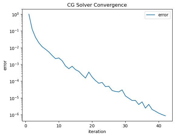
inv = solvers.CGSolver(V.mat, pre, tol=1e-6, printrates=False, plotrates=True)
gfurho = GridFunction(fesL2)
gfurho.vec.data = inv * lf.vec
<Figure size 640x480 with 0 Axes>
The solution shows strong singularities at the boundary of the shield:
[12]:
Draw (gfurho, min=-10, max=10);
[13]:
S = SingularMLExpansionCF((0,0,0), 2, 1e-10)
S.expansion.AddChargeDensity(gfurho, mesh.Boundaries(".*"))
S.expansion.Calc()
R = RegularMLExpansionCF(S, (0,0,0.00),r=5)
Draw (R.real*CF((0,0,1)), vismesh, min=-1,max=1, order=2);
[ ]:
[ ]: