This page was generated from unit-8.3-cutfem/cutfem.ipynb.

8.3 Unfitted FEM discretizations

We want to solve a geometrically unfitted model problem for a stationary domain.

We use a level set description (cf. basics.ipynb):

\[\Omega_{-} := \{ \phi < 0 \}, \quad \Omega_{+} := \{ \phi > 0 \}, \quad \Gamma := \{ \phi = 0 \}.\]

and use a piecewise linear approximation as a starting point in the discretization (cf. intlset.ipynb for a discussion of geometry approximations).

We first import the related packages:

# the constant pi
from math import pi
# ngsolve stuff
from ngsolve import *
# basic xfem functionality
from xfem import *
# basic geometry features (for the background mesh)
from netgen.geom2d import SplineGeometry
# visualization stuff
from ngsolve.webgui import *

importing ngsxfem-2.1.2405.dev0

Interface problem

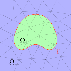
We want to solve a problem of the form:

\[\begin{split}\left\{ \begin{aligned} - \nabla \cdot (\alpha_{\pm} \nabla u) = & \, f & & \text{in}~~ \Omega_{\pm}, \\ [\![u]\!] = & \, 0 & & \text{on}~~ \Gamma, \\ [\![-\alpha \nabla u \cdot \mathbf{n}]\!] = & \, 0 & & \text{on}~~ \Gamma, \\ u = & \, u_D & & \text{on}~~ \partial \Omega. \end{aligned} \right.\end{split}\]

square = SplineGeometry()
square.AddRectangle([-1.5,-1.5],[1.5,1.5],bc=1)
mesh = Mesh (square.GenerateMesh(maxh=0.4, quad_dominated=False))

levelset = (sqrt(x*x+y*y) - 1.0)
DrawDC(levelset, -3.5, 2.5, mesh,"levelset")

lsetp1 = GridFunction(H1(mesh,order=1))
InterpolateToP1(levelset,lsetp1)
DrawDC(lsetp1, -3.5, 2.5, mesh, "lsetp1")

BaseWebGuiScene

Cut FE spaces

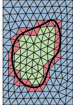
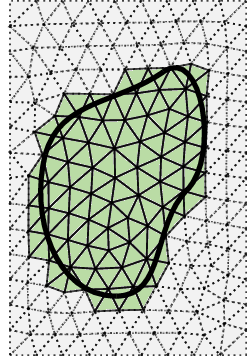
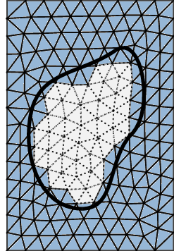
For the discretization we use standard background FESpaces restricted to the subdomains:

\[V_h^\Gamma \quad = \qquad V_h |_{\Omega_-^{lin}} \quad \oplus \quad V_h |_{\Omega_+^{lin}}\]

composed	inner	outer

In NGSolve we simply take the product space \(V_h \times V_h\) but mark the irrelevant dofs using the CutInfo-class:

Vh = H1(mesh, order=2, dirichlet=".*")
VhG = FESpace([Vh,Vh])

ci = CutInfo(mesh, lsetp1)
freedofs = VhG.FreeDofs()
freedofs &= CompoundBitArray([GetDofsOfElements(Vh,ci.GetElementsOfType(HASNEG)),
                              GetDofsOfElements(Vh,ci.GetElementsOfType(HASPOS))])

gfu = GridFunction(VhG)

Let us visualize active dofs:

• active dofs of first space are set to -1

• active dofs of second space are set to 1

• inactive dofs are 0

gfu.components[0].Set(CoefficientFunction(-1))
gfu.components[1].Set(CoefficientFunction(1))
for i, val in enumerate(freedofs):
    if not val:
        gfu.vec[i] = 0.0

Draw(gfu.components[0], mesh, "background_uneg")

BaseWebGuiScene

Draw(gfu.components[1], mesh, "background_upos")

BaseWebGuiScene

Only the parts which are in the corresponding subdomain are relevant. The solution \(u\) is:

\[\begin{split}u = \left\{ \begin{array}{cc} u_- & \text{ if } {\phi}_h^{lin} < 0, \\ u_+ & \text{ if } {\phi}_h^{lin} \geq 0. \end{array} \right.\end{split}\]

DrawDC(lsetp1, gfu.components[0], gfu.components[1], mesh, "u")

BaseWebGuiScene

Improvement: use Compress to reduce unused dofs

Vh = H1(mesh, order=2, dirichlet=[1,2,3,4])
ci = CutInfo(mesh, lsetp1)
VhG = FESpace([Compress(Vh,GetDofsOfElements(Vh,ci.GetElementsOfType(cdt))) for cdt in [HASNEG,HASPOS]])

freedofs = VhG.FreeDofs()
gfu = GridFunction(VhG)
gfu.components[0].Set(1)
gfu.components[1].Set(-1)
DrawDC(lsetp1, gfu.components[0], gfu.components[1], mesh, "u")
print(Vh.ndof, VhG.components[0].ndof, VhG.components[1].ndof)

281 136 256

Nitsche discretization

For the discretization of the interface problem we consider the Nitsche formulation:

\[\begin{split}\begin{aligned} \sum_{i \in \{+,-\}} & \left( \alpha_i \nabla u \nabla v \right)_{\Omega_i} + \left( \{\!\!\{ - \alpha \nabla u \cdot n \}\!\!\}, [\![v]\!] \right)_\Gamma + \left( [\![u]\!],\{\!\!\{ - \alpha \nabla v \cdot n \}\!\!\} \right)_\Gamma + \left( \frac{\bar{\alpha} \lambda}{h} [\![u]\!] , [\![v]\!] \right)_{\Gamma} \\ & = \left( f,v \right)_{\Omega} \end{aligned}\end{split}\]

for all \(v \in V_h^\Gamma\).

For this formulation we require:

• a suitably defined average operator \(\{ \cdot \} = \kappa_+ (\cdot)|_{\Omega_{+}} + \kappa_- (\cdot)|_{\Omega_{-}}\)

• a suitable definition of the normal direction

• numerical integration on \(\Omega_{+}^{lin}\), \(\Omega_{-}^{lin}\) and \(\Gamma^{lin}\)

Cut ratio field

For the average we use the "Hansbo"-choice:

\[\kappa_- = \frac{|T \cap \Omega_-^{lin}|}{|T|} \qquad \kappa_+ = 1 - \kappa_-\]

This "cut ratio" field is provided by the CutInfo class:

kappaminus = CutRatioGF(ci)
kappa = (kappaminus, 1-kappaminus)
Draw(kappaminus, mesh, "kappa")

BaseWebGuiScene

Normal direction

The normal direction is obtained from the (interpolated) level set function:

\[n^{lin} = \frac{\nabla \phi_h^{lin}}{\Vert \nabla \phi_h^{lin} \Vert}\]

n = Normalize(grad(lsetp1))
Draw(n, mesh, "normal", vectors={'grid_size': 20})

BaseWebGuiScene

Averages and jumps

Based on the background finite elements we can now define the averages and jumps:

h = specialcf.mesh_size

alpha = [1.0,20.0]

# Nitsche stabilization parameter:
stab = 20*(alpha[1]+alpha[0])/h

# expressions of test and trial functions (u and v are tuples):
u,v = VhG.TnT()

average_flux_u = sum([- kappa[i] * alpha[i] * grad(u[i]) * n for i in [0,1]])
average_flux_v = sum([- kappa[i] * alpha[i] * grad(v[i]) * n for i in [0,1]])

jump_u = u[0] - u[1]
jump_v = v[0] - v[1]

Integrals

To integrate only on the subdomains or the interface with a symbolic expression, you have to use the dCut differentail symbol, cf. intlset.ipynb. (Only) to speed up assembly we can mark the integrals as undefined where they would be zero anyway:

dx_neg = dCut(levelset=lsetp1, domain_type=NEG, definedonelements=ci.GetElementsOfType(HASNEG))
dx_pos = dCut(levelset=lsetp1, domain_type=POS, definedonelements=ci.GetElementsOfType(HASPOS))
ds = dCut(levelset=lsetp1, domain_type=IF, definedonelements=ci.GetElementsOfType(IF))

We first integrate over the subdomains:

\[\int_{\Omega_-} \alpha_- \nabla u \nabla v \, d\omega\]

\[\int_{\Omega_+} \alpha_+ \nabla u \nabla v \, d\omega\]

a = BilinearForm(VhG, symmetric = True)
a += alpha[0] * grad(u[0]) * grad(v[0]) * dx_neg
a += alpha[1] * grad(u[1]) * grad(v[1]) * dx_pos

We then integrate over the interface:

\[\int_{\Gamma} \{\!\!\{ - \alpha \nabla u \cdot \mathbf{n} \}\!\!\} [\![v]\!] \, d\gamma + \int_{\Gamma} \{\!\!\{ - \alpha \nabla v \cdot \mathbf{n} \}\!\!\} [\![u]\!] \, d\gamma + \int_{\Gamma} \frac{\lambda}{h} \bar{\alpha} [\![u]\!] [\![v]\!] \, d\gamma\]

a += (average_flux_u * jump_v + average_flux_v * jump_u + stab * jump_u * jump_v) * ds

Finally, we integrate over the subdomains to get the linear form:

\[f(v) = \int_{\Omega_-} f_- v \, d\omega + \int_{\Omega_+} f_+ v \, d\omega\]

coef_f = [1,0]

f = LinearForm(VhG)
f += coef_f[0] * v[0] * dx_neg
f += coef_f[1] * v[1] * dx_pos

Assembly

a.Assemble()
f.Assemble()

<ngsolve.comp.LinearForm at 0x7f94c5003b70>

We can now solve the problem (recall that freedofs only marks relevant dofs):

# homogenization of boundary data and solution of linear system
def SolveLinearSystem():
    gfu.vec[:] = 0
    f.vec.data -= a.mat * gfu.vec
    gfu.vec.data += a.mat.Inverse(freedofs) * f.vec
SolveLinearSystem()

DrawDC(lsetp1, gfu.components[0], gfu.components[1], mesh, "u", min=0, max=0.25)

BaseWebGuiScene

Higher order accuracy

In the previous example we used a second order FESpace but only used a second order accurate geometry representation (due to \(\phi_h^{lin}\)).

We can improve this by applying a mesh transformation technique, cf. intlset.ipynb:

# for isoparametric mapping
from xfem.lsetcurv import *
lsetmeshadap = LevelSetMeshAdaptation(mesh, order=2)
deformation = lsetmeshadap.CalcDeformation(levelset)
Draw(deformation, mesh, "deformation")

# alternatively to passing the deformation to dCut me can do the mesh deformation by hand
mesh.deformation = deformation
a.Assemble()
f.Assemble()
mesh.deformation = None

SolveLinearSystem()


DrawDC(lsetp1, gfu.components[0], gfu.components[1], mesh, "u", deformation=deformation, min=0, max=0.25)

uh = IfPos(lsetp1, gfu.components[1], gfu.components[0])
deform_graph = CoefficientFunction((deformation[0], deformation[1], 4*uh))
DrawDC(lsetp1, gfu.components[0], gfu.components[1], mesh, "graph_of_u", deformation=deform_graph, min=0, max=0.25)

BaseWebGuiScene

XFEM spaces

Instead of the CutFEM space

\[V_h^\Gamma = V_h |_{\Omega_-^{lin}} \oplus V_h |_{\Omega_+^{lin}}\]

we can use the (same) space with an XFEM characterization:

\[V_h^\Gamma = V_h \oplus V_h^x\]

with the space \(V_h^x\) which adds the necessary enrichments.

In ngsxfem we can also work with this XFEM spaces:

Vh = H1(mesh, order=2, dirichlet=[1,2,3,4])
Vhx = XFESpace(Vh,ci)
VhG = FESpace([Vh,Vhx])

original	after cut

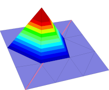
• The space Vhx copies all shape functions from Vh on cut (IF) elements (and stores a sign (NEG/POS))

• The sign determines on which domain the shape function should be supported (and where not)

• Advantage: every dof is an active dof (i.e. no dummy dofs)

• Need to express \(u_+\) and \(u_-\) in terms of \(u_h^{std}\) and \(u_h^x\):

  • \(u_- = u_h^{std} +\) neg(\(u_h^x\)) and \(u_+ = u_h^{std} +\) pos(\(u_h^x\))

• neg and pos filter out the right shape functions of Vhx

### express xfem shape functions as cutFEM shape functions:
(u_std,u_x), (v_std, v_x) = VhG.TnT()

u = [u_std + op(u_x) for op in [neg,pos]]
v = [v_std + op(v_x) for op in [neg,pos]]

Similar examples and extensions (python demo files)

In the source directory (or on http://www.github.com/ngsxfem/ngsxfem ) you can find in the demos directory a number of more advanced examples (with fewer explanatory comments). These are:

• unf_interf_prob.py : Similar to this notebook. The file implements low and high order geometry approximation and gives the choice between a CutFEM and XFEM discretisation.

• fictdom.py : Fictitious domain/CutFEM diffusion problem (one domain only) with ghost penalty stabilization.

• fictdom_dg.py : Fictitious domain/CutFEM diffusion problem with a discontiunous Galerkin discretisation and ghost-penalty stabilization.

• ficdom_mlset.py : Fictitious domain/CutFEM diffusion problem with a geometry described by multiple level set funcions.

• stokesxfem.py : Stokes interface problem with using XFEM and a Nitsche formulation.

• tracefem.py or tracefem_scalar.ipynb : A scalar Laplace-Beltrami problem on a level set surface in 3d using a trace finite element discretization (PDE on the interface only).

• lsetgeoms.py : Shows a number of pre-implemented 3d level set geometries.

• moving_domain.py : A scalar convection-diffusion problem posed on a moving domain discretised with an Eulerian time-stepping scheme.

• aggregates/fictdom_aggfem.py : Fictitious domain/CutFEM diffusion problem (one domain only) with aggregation of FE spaces

• aggregates/fictdom_dg_aggfem.py : Fictitious domain/CutFEM diffusion with DG discretization and cell aggregation

• spacetime/spacetimeCG_unfitted.py : A scalar unfitted PDE problem on a moving domain, discretized with CG-in-time space-time finite elements.

• spacetime/spacetimeDG_unfitted.py : As spacetimeCG_unfitted.py but with a DG-in-time space-time discretisation.

• spacetime/spacetimeDG_fitted.py : A fitted FEM heat equation solved using DG-in-time space-time finite elements.

• spacetime/spacetime_vtk.py : Demonstration to generate space-time VTK outputs.

• mpi/mpi_nxfem.py : Same problem as unf_interf_prob.py (XFEM + higher order) campatible with MPI parallisation.