This page was generated from appendix-vtk/vtk.ipynb.

VTK - Output

Netgen/NGSolve comes with several convenient ways to visualize your PDE solutions: the webgui, the legacy netgen GUI, … For some use cases visualization toolboxes like ParaView may still be able to obtain more insight or more complex visualizations from you computational results.

To put your results in a corresponding format you can use the VTKOutput of NGSolve.

A VTKOutput object obtains a list of coefficient functions (scalar or vector) and a list of labels. Together with the mesh information these information will be put into a vtk-formatted file on every Do-call of the object. As VTK essentially only draws piecewise linears you may want to describe a subdivision argument larger 0 to obtain higher resolution of a higher order FE function.

Let’s explore a few use cases by examples:

Example 1: single solution output

Let’s recap the Poisson solution from unit 1.1:

from ngsolve import *
from netgen.geom2d import unit_square
mesh = Mesh(unit_square.GenerateMesh(maxh=0.2))
fes = H1(mesh, order=2, dirichlet="bottom|right")
gfu = GridFunction(fes)
a = BilinearForm(fes, symmetric=True)
a += grad(fes.TrialFunction())*grad(fes.TestFunction())*dx
a.Assemble()
f = LinearForm(fes)
f += x*fes.TestFunction()*dx
f.Assemble()
gfu.vec.data = a.mat.Inverse(freedofs=fes.FreeDofs()) * f.vec

Now, instead of using the webgui, let us export the result data to a vtk file:

vtk = VTKOutput(mesh,coefs=[gfu],names=["sol"],filename="vtk_example1",subdivision=2)
vtk.Do()

'vtk_example1'

Note, only the Do()-call writes the output. Let’s see what we got:

!ls -lh vtk_example1*

-rw-rw-r-- 1 root root 303K Dec  4 02:03 vtk_example1.png
-rw-r--r-- 1 root root  36K Dec  4 02:26 vtk_example1.vtu

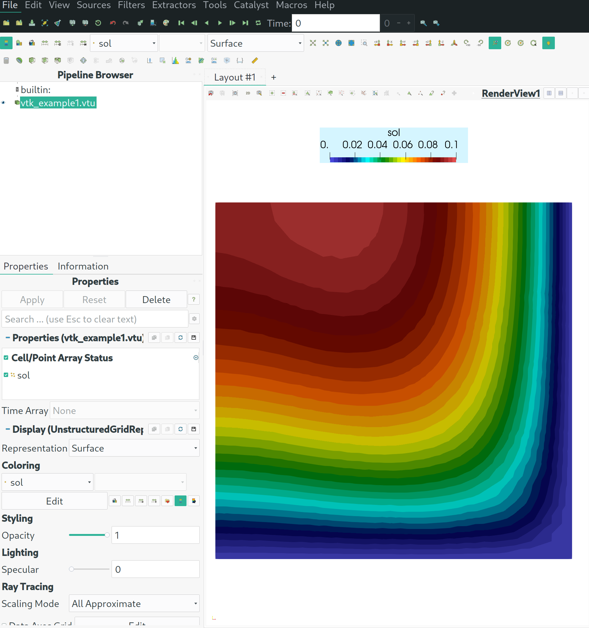
We obtained the file vtk_example1.vtu. This file can be opened with ParaView, e.g. with paraview vtk_example1.vtu where you can select your solution field and use several "filters" to process the data to get nice visualizations as the following:

You can now play around with tools like paraview to do many different complex operations.

Example 2: Series of data

In some cases you may want to analyse a sequence of simulation, e.g. for generating a video. In this case, you simply call Do() several times. You can also provide an additional time stamp with e.g. Do(time=0.3).

Let’s take a time-dependent coefficient function and put this to a sequence of VTK outputs:

t = Parameter(0)
coef = sin(4*(x+y+t))
vtkout = VTKOutput(mesh,coefs=[coef],names=["sol"],filename="vtk_example2",subdivision=2)
vtkout.Do(time = 0.0)
for i in range(20):
    t.Set((i+1)/20)
    vtkout.Do(time = (i+1)/20.0)

Let’s see what we got this time:

ls -lh vtk_example2*

-rw-rw-r-- 1 root root 350K Dec  4 02:03 vtk_example2.png
-rw-r--r-- 1 root root 1.4K Dec  4 02:26 vtk_example2.pvd
-rw-r--r-- 1 root root  36K Dec  4 02:26 vtk_example2.vtu
-rw-r--r-- 1 root root  36K Dec  4 02:26 vtk_example2_step00001.vtu
-rw-r--r-- 1 root root  36K Dec  4 02:26 vtk_example2_step00002.vtu
-rw-r--r-- 1 root root  36K Dec  4 02:26 vtk_example2_step00003.vtu
-rw-r--r-- 1 root root  36K Dec  4 02:26 vtk_example2_step00004.vtu
-rw-r--r-- 1 root root  36K Dec  4 02:26 vtk_example2_step00005.vtu
-rw-r--r-- 1 root root  36K Dec  4 02:26 vtk_example2_step00006.vtu
-rw-r--r-- 1 root root  36K Dec  4 02:26 vtk_example2_step00007.vtu
-rw-r--r-- 1 root root  36K Dec  4 02:26 vtk_example2_step00008.vtu
-rw-r--r-- 1 root root  36K Dec  4 02:26 vtk_example2_step00009.vtu
-rw-r--r-- 1 root root  36K Dec  4 02:26 vtk_example2_step00010.vtu
-rw-r--r-- 1 root root  36K Dec  4 02:26 vtk_example2_step00011.vtu
-rw-r--r-- 1 root root  36K Dec  4 02:26 vtk_example2_step00012.vtu
-rw-r--r-- 1 root root  36K Dec  4 02:26 vtk_example2_step00013.vtu
-rw-r--r-- 1 root root  36K Dec  4 02:26 vtk_example2_step00014.vtu
-rw-r--r-- 1 root root  36K Dec  4 02:26 vtk_example2_step00015.vtu
-rw-r--r-- 1 root root  36K Dec  4 02:26 vtk_example2_step00016.vtu
-rw-r--r-- 1 root root  36K Dec  4 02:26 vtk_example2_step00017.vtu
-rw-r--r-- 1 root root  36K Dec  4 02:26 vtk_example2_step00018.vtu
-rw-r--r-- 1 root root  36K Dec  4 02:26 vtk_example2_step00019.vtu
-rw-r--r-- 1 root root  36K Dec  4 02:26 vtk_example2_step00020.vtu

• We obtained 21 .vtu-files corresponding to the 21 Do-calls.

• Only the first Do-call does not have an additional suffix, while later calls append the _step...-suffix.

• Furthermore there is a .pvd file which bundles the individual files and associates them to the provided time stamps (if provided):

!cat vtk_example2.pvd

<?xml version="1.0"?>
<VTKFile type ="Collection" version="1.0" byte_order="LittleEndian">
<Collection>
<DataSet timestep="0" file="vtk_example2.vtu"/>
<DataSet timestep="0.05" file="vtk_example2_step00001.vtu"/>
<DataSet timestep="0.1" file="vtk_example2_step00002.vtu"/>
<DataSet timestep="0.15" file="vtk_example2_step00003.vtu"/>
<DataSet timestep="0.2" file="vtk_example2_step00004.vtu"/>
<DataSet timestep="0.25" file="vtk_example2_step00005.vtu"/>
<DataSet timestep="0.3" file="vtk_example2_step00006.vtu"/>
<DataSet timestep="0.35" file="vtk_example2_step00007.vtu"/>
<DataSet timestep="0.4" file="vtk_example2_step00008.vtu"/>
<DataSet timestep="0.45" file="vtk_example2_step00009.vtu"/>
<DataSet timestep="0.5" file="vtk_example2_step00010.vtu"/>
<DataSet timestep="0.55" file="vtk_example2_step00011.vtu"/>
<DataSet timestep="0.6" file="vtk_example2_step00012.vtu"/>
<DataSet timestep="0.65" file="vtk_example2_step00013.vtu"/>
<DataSet timestep="0.7" file="vtk_example2_step00014.vtu"/>
<DataSet timestep="0.75" file="vtk_example2_step00015.vtu"/>
<DataSet timestep="0.8" file="vtk_example2_step00016.vtu"/>
<DataSet timestep="0.85" file="vtk_example2_step00017.vtu"/>
<DataSet timestep="0.9" file="vtk_example2_step00018.vtu"/>
<DataSet timestep="0.95" file="vtk_example2_step00019.vtu"/>
<DataSet timestep="1" file="vtk_example2_step00020.vtu"/>
</Collection>
</VTKFile>

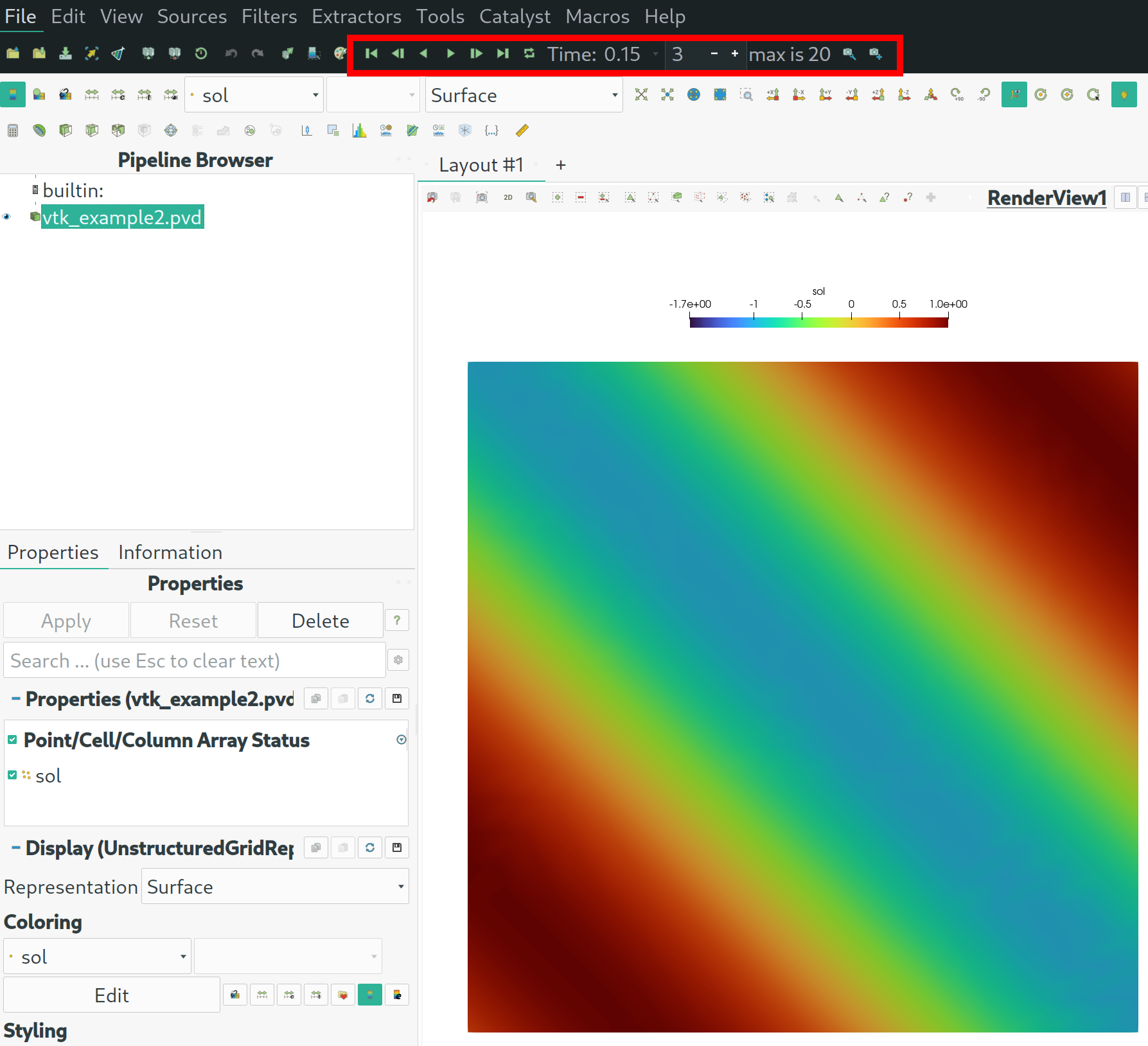
Now you can open this "meta file" with paraview and visualize the time series with many different filter. Finally, you can export stills or videos from that. It will look like this:

Further options

To learn more about possible options you show call help(VTKOutput). Nevertheless, let us comment on a few of theme:

• VTKOutput(..., subdivision=i) refines the mesh (locally and only temporarily) as often as i. Note that when opened with ParaView the visualized mesh no longer coincides with your computational mesh.

• VTKOutput(..., only_element=i) puts only the data of one selected element out. This can be interesting for basis function visualization or alike.

• VTKOutput(..., floatsize=fs) where fs is either "single" or "double" decides on the precision of the output. Default is "double". Using "single" can significantly reduce the used disk space.

there are further options for the Do(...)-call that we briefly discuss:

• ....Do(time=t) adds the time stamp t to the meta-file if a series of outputs is used.

• ....Do(vb=vb) allows you to switch from volume mesh output (vb=VOL, default) to surface mesh output (vb=BND)

• ....Do(drawelems=els) allows you to only write a submesh of the underlying mesh where the corresponding set of elements is prescribed by the BitArray els.

help(VTKOutput)

Help on class VTKOutput in module ngsolve.comp:

class VTKOutput(pybind11_builtins.pybind11_object)
 |  Method resolution order:
 |      VTKOutput
 |      pybind11_builtins.pybind11_object
 |      builtins.object
 |
 |  Methods defined here:
 |
 |  Do(...)
 |      Do(*args, **kwargs)
 |      Overloaded function.
 |
 |      1. Do(self: ngsolve.comp.VTKOutput, time: float = -1, vb: ngsolve.comp.VorB = <VorB.VOL: 0>) -> str
 |
 |
 |      Write mesh and fields to file. When called several times on the same object
 |      an index is added to the output file name. A meta file (.pvd) is written
 |      (unless in legacy mode).
 |
 |      Returns string of the output filename.
 |
 |      Parameters:
 |
 |      time :
 |        associate a time to the current output
 |
 |      vb: VOL_or_BND (default VOL)
 |        defines if output is done on the volume (VOL) or surface mesh (BND).
 |                  .
 |
 |      2. Do(self: ngsolve.comp.VTKOutput, time: float = -1, vb: ngsolve.comp.VorB = <VorB.VOL: 0>, drawelems: pyngcore.pyngcore.BitArray) -> str
 |
 |
 |      Write mesh and fields to file. When called several times on the same object
 |      an index is added to the output file name. A meta file (.pvd) is written
 |      (unless in legacy mode).
 |
 |      Returns string of the output filename.
 |
 |      Parameters:
 |
 |      time :
 |        associate a time to the current output (default: output counter)
 |
 |      vb: VOL_or_BND (default VOL)
 |        defines if output is done on the volume (VOL) or surface mesh (BND).
 |
 |      drawelems: BitArray
 |        defines the submesh (set of elements) that are (only) used for drawing.
 |                  .
 |
 |  __init__(...)
 |      __init__(self: ngsolve.comp.VTKOutput, ma: ngsolve.comp.Mesh, coefs: list = [], names: list = [], filename: str = 'vtkout', subdivision: int = 0, only_element: int = -1, floatsize: str = 'double', legacy: bool = False, order: int = 1) -> None
 |
 |
 |      VTK output class. Allows to put mesh and field information of several CoefficientFunctions into a VTK file.
 |      (Can be used by independent visualization software, e.g. ParaView).
 |
 |      When run in parallel, rank 0 stores no vtk output, but writes the pvd-file that links all parallel
 |      output together.
 |
 |      Parameters:
 |
 |      ma : ngsolve mesh
 |        mesh (Note: if a deformation is set, the output will be w.r.t. the deformed state of the mesh)
 |
 |      coefs: list of CoefficientFunctions
 |        list of CFs that are stored as fields in the Paraview output
 |
 |      names : list of strings
 |        labels for the fields that are put in the output file
 |
 |      filename : string (default: \"output\")
 |        name of the output file ( .vtu file ending is added or .vtk file ending is added (legacy mode) ).
 |        If run in parallel, the suffix \"_procxyz\" is added (xyz a number).
 |        If output is written several times, the ending \"_stepxyz\" is added (xyz a counter).
 |        If run in parallel or the output is called several times a meta file with ending .pvd is also generated for convenience.
 |
 |      subdivision : int
 |        Number of subdivision (bisections in each direction) that are applied
 |        (Note that only vertex values are stored otherwise rendering the output information piecewise linear only)
 |
 |      only_element : int
 |        only work on one specific element (default: -1 which means `draw all elements`)
 |
 |      floatsize : string in {\"single\", \"double\" }   object
 |        defines the precision of the output data (default is \"double\", \"single\" can be used to reduce output)
 |
 |      legacy : bool (default: False)
 |        defines if legacy-VTK output shall be used
 |
 |      order : int (default: 1)
 |        allowed values: 1,2
 |                  .
 |
 |  ----------------------------------------------------------------------
 |  Static methods inherited from pybind11_builtins.pybind11_object:
 |
 |  __new__(*args, **kwargs) class method of pybind11_builtins.pybind11_object
 |      Create and return a new object.  See help(type) for accurate signature.