This page was generated from unit-1.6-adaptivity/adaptivity.ipynb.

1.6 Error estimation & adaptive refinement

In this tutorial, we apply a Zienkiewicz-Zhu type error estimator and run an adaptive loop with these steps:

\[\text{SOLVE}\rightarrow \text{ESIMATE}\rightarrow \text{MARK}\rightarrow \text{REFINE}\rightarrow \text{SOLVE} \rightarrow \ldots\]

from ngsolve import *
from ngsolve.webgui import Draw
from netgen.occ import *
import matplotlib.pyplot as plt

Geometry

The following geometry represents a heated chip embedded in another material that conducts away the heat.

def MakeGeometryOCC():
    base = Rectangle(1, 0.6).Face()
    chip = MoveTo(0.5,0.15).Line(0.15,0.15).Line(-0.15,0.15).Line(-0.15,-0.15).Close().Face()
    top = MoveTo(0.2,0.6).Rectangle(0.6,0.2).Face()
    base -= chip

    base.faces.name="base"
    chip.faces.name="chip"
    chip.faces.col=(1,0,0)
    top.faces.name="top"
    geo = Glue([base,chip,top])
    geo.edges.name="default"
    geo.edges.Min(Y).name="bot"
    return OCCGeometry(geo, dim=2)

mesh = Mesh(MakeGeometryOCC().GenerateMesh(maxh=0.2))
Draw(mesh)

BaseWebGuiScene

Spaces & forms

The problem is to find \(u\) in \(H_{0,D}^1\) satisfying

\[\int_\Omega \lambda \nabla u \cdot \nabla v = \int_\Omega f v\]

for all \(v\) in \(H_{0,D}^1\). We expect the solution to have singularities due to the nonconvex re-enrant angles and discontinuities in \(\lambda\).

fes = H1(mesh, order=3, dirichlet=[1])
u, v = fes.TnT()

# one heat conductivity coefficient per sub-domain
lam = CoefficientFunction([1, 1000, 10])
a = BilinearForm(lam*grad(u)*grad(v)*dx)

# heat-source in inner subdomain
f = LinearForm(fes)
f = LinearForm(1*v*dx(definedon="chip"))

c = Preconditioner(a, type="multigrid", inverse="sparsecholesky")

gfu = GridFunction(fes)

Note that the linear system is not yet assembled above.

Solve

Since we must solve multiple times, we define a function to solve the boundary value problem, where assembly, update, and solve occurs.

def SolveBVP():
    fes.Update()
    gfu.Update()
    a.Assemble()
    f.Assemble()
    inv = CGSolver(a.mat, c.mat)
    gfu.vec.data = inv * f.vec

SolveBVP()
Draw(gfu);

Estimate

We implement a gradient-recovery-type error estimator. For this, we need an H(div) space for flux recovery. We must compute the flux of the computed solution and interpolate it into this H(div) space.

space_flux = HDiv(mesh, order=2)
gf_flux = GridFunction(space_flux, "flux")

flux = lam * grad(gfu)
gf_flux.Set(flux)

Element-wise error estimator: On each element \(T\), set

\[\eta_T^2 = \int_T \frac{1}{\lambda} |\lambda \nabla u_h - I_h(\lambda \nabla u_h) |^2\]

where \(u_h\) is the computed solution gfu and \(I_h\) is the interpolation performed by Set in NGSolve.

err = 1/lam*(flux-gf_flux)*(flux-gf_flux)
Draw(err, mesh, 'error_representation')

BaseWebGuiScene

eta2 = Integrate(err, mesh, VOL, element_wise=True)
print(eta2)

 5.80014e-10
 7.49183e-08
 8.51912e-06
 4.54368e-10
 8.33308e-08
 4.83986e-09
 3.08064e-07
 7.02005e-10
 1.1091e-08
 3.03261e-08
 1.0408e-07
 2.48804e-07
 7.10938e-08
 8.58958e-07
 7.75911e-06
 1.01521e-06
 6.85467e-08
 7.87624e-06
 2.05199e-06
 2.25556e-08
 1.65616e-07
 6.07265e-08
 1.74824e-06
 1.18772e-06
 3.46568e-07
 2.52966e-06
 1.46647e-09
 1.88656e-06
 1.17887e-06
 4.09713e-08
 1.57525e-07
 1.60365e-09
 1.92225e-08
 1.9544e-08
 1.14778e-09
 9.56943e-10
 6.7901e-09
 8.51976e-10
 1.44089e-10
 9.55771e-09

The above values, one per element, lead us to identify elements which might have large error.

Mark

We mark elements with large error estimator for refinement.

maxerr = max(eta2)
print ("maxerr = ", maxerr)

for el in mesh.Elements():
    mesh.SetRefinementFlag(el, eta2[el.nr] > 0.25*maxerr)
    # see below for vectorized alternative

maxerr =  8.519121326541049e-06

Refine & solve again

Refine marked elements:

mesh.Refine()
SolveBVP()
Draw(gfu)

BaseWebGuiScene

Automate the above steps

l = []    # l = list of estimated total error

def CalcError():

    # compute the flux:
    space_flux.Update()
    gf_flux.Update()
    flux = lam * grad(gfu)
    gf_flux.Set(flux)

    # compute estimator:
    err = 1/lam*(flux-gf_flux)*(flux-gf_flux)
    eta2 = Integrate(err, mesh, VOL, element_wise=True)
    maxerr = max(eta2)
    l.append ((fes.ndof, sqrt(sum(eta2))))
    print("ndof =", fes.ndof, " maxerr =", maxerr)

    # mark for refinement (vectorized alternative)
    mesh.ngmesh.Elements2D().NumPy()["refine"] = eta2.NumPy() > 0.25*maxerr

CalcError()
mesh.Refine()

ndof = 328  maxerr = 5.0385892733977e-06

Run the adaptive loop

level = 0
while fes.ndof < 50000:
    SolveBVP()
    level = level + 1
    if level%5 == 0:
        print('adaptive step #', level)
        Draw(gfu)
    CalcError()
    mesh.Refine()

ndof = 583  maxerr = 2.0247198934825063e-06
ndof = 997  maxerr = 8.0374929330418e-07
ndof = 1492  maxerr = 3.1888429487698495e-07
ndof = 2143  maxerr = 1.264974505886916e-07
adaptive step # 5

ndof = 2917  maxerr = 5.01634985327537e-08
ndof = 3775  maxerr = 1.988922745586041e-08
ndof = 4651  maxerr = 8.08369538279698e-09
ndof = 5440  maxerr = 3.86423125252989e-09
ndof = 6211  maxerr = 1.8513183508753528e-09
adaptive step # 10

ndof = 6910  maxerr = 8.88018609108649e-10
ndof = 7456  maxerr = 4.2622762648173923e-10
ndof = 8263  maxerr = 2.0464796527367645e-10
ndof = 9433  maxerr = 9.827590625263762e-11
ndof = 10495  maxerr = 4.719861824266745e-11
adaptive step # 15

ndof = 12130  maxerr = 2.2668856545775322e-11
ndof = 13675  maxerr = 1.0887894643432407e-11
ndof = 15259  maxerr = 5.229541399463823e-12
ndof = 18055  maxerr = 2.5117726640897505e-12
ndof = 20347  maxerr = 1.2064449409699737e-12
adaptive step # 20

ndof = 23761  maxerr = 5.79460999395933e-13
ndof = 27262  maxerr = 2.7832639279306787e-13
ndof = 31426  maxerr = 1.3367946296920183e-13
ndof = 37588  maxerr = 6.420965229814459e-14
ndof = 43645  maxerr = 3.0839098645895766e-14

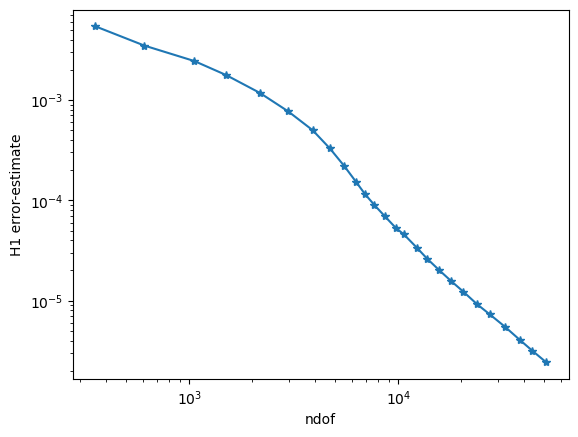
Plot history of adaptive convergence

plt.yscale('log')
plt.xscale('log')
plt.xlabel("ndof")
plt.ylabel("H1 error-estimate")
ndof,err = zip(*l)
plt.plot(ndof,err, "-*")

plt.ion()
plt.show()