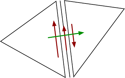
3.6 DG/HDG splitting
When solving unsteady problems with an operator-splitting method it might be benefitial to consider different space discretizations for different operators.
For a problem of the form
We consider the operator splitting:
- 1.Step: Given \(u^0\), solve \(t^n \to t^{n+1}\): \(\quad \partial_t u + C u = 0 \Rightarrow u^{\frac12}\)
- 2.Step: Given \(u^{\frac12}\), solve \(t^n \to t^{n+1}\): \(\quad \partial_t u + A u = 0 \Rightarrow u^{1}\)
This splitting is only first order accurate but allows to take different time discretizations for the substeps 1 and 2.
In this example we consider the Navier-Stokes problem again (cf. 3.2) and want to combine
- an \(H(div)\) -conforming Hybrid DG method (which is a very good discretization for Stokes-type problems) and
- a standard upwind DG method for the discretization of the convection
The weak form is: Find \((\mathbf{u},p):[0,T] \to (H_{0,D}^1)^d \times L^2\), s.t.
Again, we consider the benchmark setup from http://www.featflow.de/en/benchmarks/cfdbenchmarking/flow/dfg_benchmark2_re100.html . The geometry:

The viscosity is set to \(\nu = 10^{-3}\).
In [1]:
import netgen.gui
%gui tk
from math import pi
from ngsolve import *
from netgen.geom2d import SplineGeometry
geo = SplineGeometry()
geo.AddRectangle( (0, 0), (2, 0.41), bcs = ("wall", "outlet", "wall", "inlet") )
geo.AddCircle ( (0.2, 0.2), r=0.05, leftdomain = 0, rightdomain = 1, bc = "cyl" )
mesh = Mesh( geo.GenerateMesh(maxh = 0.08) )
order = 3
mesh.Curve(order)
For the HDG formulation we use the product space with
- \(BDM_k\): \(H(div)\) conforming FE space (degree k)
- Vector facet space: facet functions of degree k (vector valued and only in tangential direction)
- piecewise polynomials up to degree \(k-1\) for the pressure

HDG spaces
In [2]:
V1 = HDiv ( mesh, order = order, dirichlet = "wall|cyl|inlet" )
V2 = FESpace ( "vectorfacet", mesh, order = order, dirichlet = "wall|cyl|inlet" )
Q = L2( mesh, order = order-1)
V = FESpace ([V1,V2,Q])

u, uhat, p = V.TrialFunction()
v, vhat, q = V.TestFunction()
Stokes discretization / initial conditions
The bilinear form to the HDG discretized Stokes problem is:
where \([\cdot]_t\) is the tangential projection of the jump \((\cdot)_T - (\cdot)_F\).
The mass matrix is simply
In [3]:
nu = 0.001
alpha = 4

gradu = CoefficientFunction ( (grad(u),), dims=(2,2) )
gradv = CoefficientFunction ( (grad(v),), dims=(2,2) )

n = specialcf.normal(mesh.dim)
h = specialcf.mesh_size

def tang(vec):
    return vec - (vec*n)*n

a = BilinearForm ( V, symmetric=True)
a += SymbolicBFI ( nu*InnerProduct ( gradu, gradv) )
a += SymbolicBFI ( nu*InnerProduct ( gradu.trans * n,  tang(vhat-v) ), element_boundary=True )
a += SymbolicBFI ( nu*InnerProduct ( gradv.trans * n,  tang(uhat-u) ), element_boundary=True )
a += SymbolicBFI ( nu*alpha*order*order/h * InnerProduct ( tang(vhat-v),  tang(uhat-u) ), element_boundary=True )
a += SymbolicBFI ( -div(u)*q -div(v)*p )
a.Assemble()

m = BilinearForm(V , symmetric=True)
m += SymbolicBFI( u * v )
m.Assemble()

f = LinearForm ( V )
As initial condition we solve the Stokes problem:
In [4]:
gfu = GridFunction(V)

U0 = 1.5
uin = CoefficientFunction( (U0*4*y*(0.41-y)/(0.41*0.41),0) )
gfu.components[0].Set(uin, definedon=mesh.Boundaries("inlet"))


invstokes = a.mat.Inverse(V.FreeDofs(), inverse="umfpack")

res = f.vec.CreateVector()
res.data = f.vec - a.mat*gfu.vec
gfu.vec.data += invstokes * res

Draw( gfu.components[0], mesh, "velocity" )
Draw( Norm(gfu.components[0]), mesh, "absvel(hdiv)")
Application of convection
In the operator splitted approach we want to apply only operator applications for the convection part. Further, we want to do this in a usual DG setting. As a model problem we use the following procedure:
- Given \((\mathbf{u},p)\) in HDG space: project into \(\hat{\mathbf{u}}\) in usual DG space
- Solve \(\partial_t \hat{\mathbf{u}} = C \hat{\mathbf{u}}\) by explicit scheme (involves convection evaluations and mass matrix operations only)
- Solve Unsteady Stokes step with r.h.s. from convection sub-problem. To this end evaluate mixed mass matrix \(\int \hat{\mathbf{u}} \cdot \mathbf{v}\) to obtain a functional on the HDG space
For the projection steps we use mixed mass matrices:
- \(M_m\) : \(HDG \times DG \to \mathbb{R}\)
- \(M_m^T\) : \(DG \times HDG \to \mathbb{R}\)
- \(M_{DG}\) : \(DG \times DG \to \mathbb{R}\) (block diagonal)
mixed mass matrices
To set up mixed mass matrices we use a bilinear form with two different FESpaces.
We do not assemble the matrices as we will only need the matrix-vector applications of \(M_m\), \(M_m^T\) and \(M_{DG}^{-1}\).
In [5]:
VL2 = L2(mesh, dim=mesh.dim, order=order)
uL2 = VL2.TrialFunction()
vL2 = VL2.TestFunction()

gfuL2 = GridFunction(VL2)

bfmixed = BilinearForm ( V, VL2, nonassemble=True )
bfmixed += SymbolicBFI ( vL2*u )

bfmixedT = BilinearForm ( VL2, V, nonassemble=True)
bfmixedT += SymbolicBFI ( uL2*v )
convection operator
- convection operation with standard Upwinding
- No set up of the matrix (only interested in operator applications)
- for the advection velocity we use the \(H(div)\)-conforming velocity (which is pointwise divergence free).
In [6]:
vel = gfu.components[0]
convL2 = BilinearForm(VL2, nonassemble=True )
convL2 += SymbolicBFI( (-InnerProduct(grad(vL2).trans * vel, uL2.trans)) )
un = InnerProduct(vel,n)
upwindL2 = IfPos(un, un*uL2, un*uL2.Other(bnd=uin))
convL2 += SymbolicBFI( InnerProduct (upwindL2, vL2-vL2.Other()), VOL, skeleton=True )
convL2 += SymbolicBFI( InnerProduct (upwindL2, vL2), BND, skeleton=True )
solution of convection steps
We now define the solution of the convection problem for an initial data \(u\) in the HDG space. The return value (“res”) is \(M_m \hat{u}\) where \(\hat{u}\) is the solution of several explicit Euler steps of the convection problem
In [7]:
def SolveConvectionSteps(gfuvec, res, tau, steps):
    bfmixed.Apply (gfuvec, gfuL2.vec)
    VL2.SolveM(gfuL2.vec, CoefficientFunction(1))
    conv_applied = gfuL2.vec.CreateVector()
    for i in range(steps):
        convL2.Apply(gfuL2.vec,conv_applied)
        VL2.SolveM(conv_applied, CoefficientFunction(1))
        gfuL2.vec.data -= tau/steps * conv_applied
        #Redraw()
    bfmixedT.Apply (gfuL2.vec, res)

#SolveConvectionSteps(gfu,res,0.01,1)
#Draw(gfuL2, mesh, "velocity(L2)")
#Draw(Norm(gfuL2), mesh, "absvel(L2)")
Operator splitting method
In [8]:
# initial values again:
res.data = f.vec - a.mat*gfu.vec
gfu.vec.data += invstokes * res
t = 0
tend = 0
In [9]:
tend += 1
substeps = 10
tau = 0.01

mstar = m.mat.CreateMatrix()
mstar.AsVector().data = m.mat.AsVector() + tau * a.mat.AsVector()
inv = mstar.Inverse(V.FreeDofs(), inverse="umfpack")

while t < tend:
    SolveConvectionSteps(gfu.vec, res, tau, substeps)
    res.data -= mstar * gfu.vec
    gfu.vec.data += inv * res
    t += tau
    print ("\r  t =", t, end="")
    Redraw(blocking=True)
t = 1.000000000000000775