This page was generated from wta/adaptivity.ipynb.
Adaptivity
[1]:
from ngsolve import *
from netgen.occ import *
from ngsolve.webgui import Draw
Define the geometry by 2D Netgen-OpenCascade modeling: Define rectangles and polygones, and glue them together to one shape object. OCC maintains the full geometry topology of vertices, edges, faces and solids.
[2]:
def MakeGeometry():
base = Rectangle(1, 0.6).Face()
chip = MoveTo(0.5,0.15).Line(0.15,0.15).Line(-0.15,0.15).Line(-0.15,-0.15).Close().Face()
top = MoveTo(0.2,0.6).Rectangle(0.6,0.2).Face()
base -= chip
base.faces.name="base"
chip.faces.name="chip"
chip.faces.col=(1,0,0)
top.faces.name="top"
geo = Glue([base,chip,top])
geo.edges.name="default"
geo.edges.Min(Y).name="bot"
Draw(geo)
return geo
geo = MakeGeometry()
Piece-wise constant coefficients in sub-domains:
[3]:
mesh = geo.GenerateMesh(maxh=0.2, dim=2)
print (mesh.GetMaterials())
('base', 'chip', 'top')
[4]:
fes = H1(mesh, order=3, dirichlet="bot")
u, v = fes.TnT()
lam = mesh.MaterialCF( { "base" : 1, "chip" : 1000, "top" : 20 } )
a = BilinearForm(lam*grad(u)*grad(v)*dx)
# heat-source in inner subdomain
f = LinearForm(1*v*dx(definedon="chip"))
c = preconditioners.MultiGrid(a, inverse="sparsecholesky")
gfu = GridFunction(fes)
Assemble and solve problem:
[5]:
def SolveBVP():
a.Assemble()
f.Assemble()
inv = CGSolver(a.mat, c.mat)
gfu.vec.data = inv * f.vec
SolveBVP()
Draw (gfu, mesh);
Gradient recovery error estimator: Interpolate finite element flux
\[q_h := I_h (\lambda \nabla u_h)\]
and take difference as element error indicator:
\[\eta_T := \tfrac{1}{\lambda} \| q_h - \lambda \nabla u_h \|_{L_2(T)}^2\]
[6]:
l = [] # list of dofs and estimated total error
gf_flux = GridFunction(HDiv(mesh, order=2))
def CalcError():
flux = lam * grad(gfu) # the FEM-flux
gf_flux.Set(flux) # interpolate into H(div)
# compute estimator:
err = 1/lam*(flux-gf_flux)*(flux-gf_flux)
eta2 = Integrate(err, mesh, VOL, element_wise=True)
l.append ((fes.ndof, sqrt(sum(eta2))))
print("ndof =", fes.ndof, " toterr =", sqrt(sum(eta2)))
# mark elements for refinement using numpy vectorization
mesh.ngmesh.Elements2D().NumPy()["refine"] = eta2.NumPy() > 0.25*max(eta2)
CalcError()
ndof = 208 toterr = 0.0062109017000810405
Adaptive loop:
[7]:
level = 0
while fes.ndof < 50000:
mesh.Refine()
SolveBVP()
CalcError()
level = level+1
if level%5 == 0:
Draw (gfu)
ndof = 328 toterr = 0.005434323802496817
ndof = 583 toterr = 0.0034474161171851457
ndof = 997 toterr = 0.0024776272650126425
ndof = 1492 toterr = 0.001764188013719247
ndof = 2158 toterr = 0.00117589425643559
ndof = 2950 toterr = 0.000772068501319359
ndof = 3826 toterr = 0.0005050543888609081
ndof = 4651 toterr = 0.00033457393100887927
ndof = 5422 toterr = 0.00022627521650948952
ndof = 6121 toterr = 0.00015855832952377152
ndof = 6586 toterr = 0.00012787178850998902
ndof = 7321 toterr = 9.644005521457746e-05
ndof = 8200 toterr = 7.791024979147798e-05
ndof = 9184 toterr = 6.082708443703687e-05
ndof = 9895 toterr = 5.020406998270656e-05
ndof = 11209 toterr = 3.91352520749997e-05
ndof = 12994 toterr = 2.8053692395244727e-05
ndof = 14365 toterr = 2.3273511700729243e-05
ndof = 16252 toterr = 1.8486318278239676e-05
ndof = 18613 toterr = 1.4268464429483311e-05
ndof = 21763 toterr = 1.0776539402620024e-05
ndof = 25099 toterr = 8.414670493706427e-06
ndof = 28927 toterr = 6.56100575423594e-06
ndof = 33445 toterr = 5.037685792056461e-06
ndof = 38899 toterr = 3.844396993226533e-06
ndof = 45985 toterr = 2.9011699121116974e-06
ndof = 53179 toterr = 2.2778128479088826e-06
[8]:
Draw (gfu);
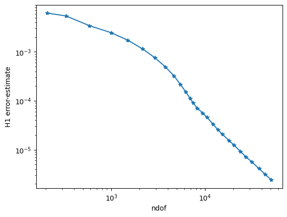
Plotting convergence:
[9]:
%matplotlib inline
import matplotlib.pyplot as plt
plt.yscale('log')
plt.xscale('log')
plt.xlabel("ndof")
plt.ylabel("H1 error-estimate")
ndof,err = zip(*l)
plt.plot(ndof,err, "-*")
plt.ion()
plt.show();
[ ]: