This page was generated from unit-7-optimization/05_Topological_Derivative_Transmission.ipynb.
7.7 PDE-Constrained Topology Optimization
We are again interested in minimizing a shape function of the type
subject to \(u:\mathsf{D} \to \mathbb{R}\) solves
where
\(\beta_\Omega = \beta_1\chi_\Omega + \beta_2 \chi_{\mathsf{D}\setminus \Omega}\), \(\qquad \beta_1,\beta_2>0\),
\(f_\Omega = f_1\chi_\Omega + f_2 \chi_{\mathsf{D}\setminus \Omega}\), \(\qquad f_1,f_2\in \mathbb{R}\),
\(u_d:\mathsf{D} \to \mathbb{R}\).
[1]:
from netgen.geom2d import SplineGeometry  # SplieGeometry to define a 2D mesh

from ngsolve import * # import everything from the ngsolve module
from ngsolve.webgui import Draw

import numpy as np

from interpolations import InterpolateLevelSetToElems # function which interpolates a levelset function

myMAXH = 0.05
EPS = myMAXH * 1e-6      #variable defining when a point is on the interface and when not
The file interpolations.py can contains a routine to compute the volume ratio of each element with respect to a given level set function. The file can be downloaded from interpolations.py .
We begin with defining the domain \(\mathsf{D}\). For this we define a rectangular mesh with side length \(R\) using the NGSolve function SplineGeometry() with maximum triangle size maxh. The boundary name of \(\partial\mathsf{D}\) is “rectangle”.
[2]:
geo = SplineGeometry()

R = 2

## add a rectangle
geo.AddRectangle(p1=(-R,-R),
                 p2=(R,R),
                 bc="rectangle",
                 leftdomain=1,
                 rightdomain=0)


geo.SetMaterial (1, "outer") # give the domain the name "outer"

mesh = Mesh(geo.GenerateMesh(maxh=myMAXH)) # generate ngsolve mesh
Draw(mesh)
[2]:
BaseWebGuiScene
fes_state,fes_adj - \(H^1\) conforming finite element space of order 1
pwc - \(L^2\) subspace of functions constant on each element of mesh
\(u,v\) are our trial and test functions
gfu, gfp are Gridfunctions storing the state and adjoint variable, respectively
gfud stores \(u_d\) - the target function
[3]:
# H1-conforming finite element space

fes_state = H1(mesh, order=1, dirichlet="rectangle")
fes_adj = H1(mesh, order=1, dirichlet="rectangle")
fes_level = H1(mesh, order=1)

pwc = L2(mesh)   #piecewise constant space


## test and trial functions
u, v = fes_state.TnT()

p, q = fes_adj.TnT()

gfu = GridFunction(fes_state)
gfp = GridFunction(fes_adj)

gfud = GridFunction(fes_state)
We represent the design \(\Omega \subset \mathsf{D}\) by means of a level set function \(\psi: \mathsf{D} \rightarrow \mathbb R\) in the following way:
psi - gridfunction in fes_state defining \(\psi\)
psides - gridfunction describing the optimal shape
psinew - dummy function for line search
[4]:
psi = GridFunction(fes_level)
psi.Set(1)

psides = GridFunction(fes_level)
psinew = GridFunction(fes_level)
Next we solve the state equation \begin{equation} \int_{\mathsf{D}} \beta_\Omega \nabla u \cdot \nabla \varphi \;dx = \int_{\mathsf{D}} f_\Omega\varphi \;dx \quad \text{ for all } \varphi \in H^1_0(\mathsf{D}). \end{equation}
beta, f_rhs - piecewise constant gridfunction
B - bilinear form defining \(\int_{\mathsf{D}} \beta_\Omega\nabla \psi \cdot \nabla \varphi \;dx\)
B_adj - bilinear form defining \(\int_{\mathsf{D}} \beta_\Omega\nabla \psi \cdot \nabla \varphi \;dx\)
L - right hand side \(\int_{\mathsf{D}} f_\Omega \varphi \;dx\)
[5]:
# constants for f_rhs and beta
f1 = 10
f2 = 1

beta1 = 10
beta2 = 1

# piecewise constant coefficient functions beta and f_rhs

beta = GridFunction(pwc)
beta.Set(beta1)

f_rhs = GridFunction(pwc)
f_rhs.Set(f1)

# bilinear form for state equation
B = BilinearForm(fes_state)
B += beta*grad(u) * grad(v) * dx

B_adj = BilinearForm(fes_adj)
B_adj += beta*grad(p) * grad(q) * dx

L = LinearForm(fes_state)
L += f_rhs * v *dx

duCost = LinearForm(fes_adj)

# solving
psides.Set(1)
InterpolateLevelSetToElems(psides, beta1, beta2, beta, mesh, EPS)
InterpolateLevelSetToElems(psides, f1, f2, f_rhs, mesh, EPS)

B.Assemble()
L.Assemble()

inv = B.mat.Inverse(fes_state.FreeDofs(), inverse="sparsecholesky") # inverse of bilinear form
gfu.vec.data = inv*L.vec

scene_u = Draw(gfu)
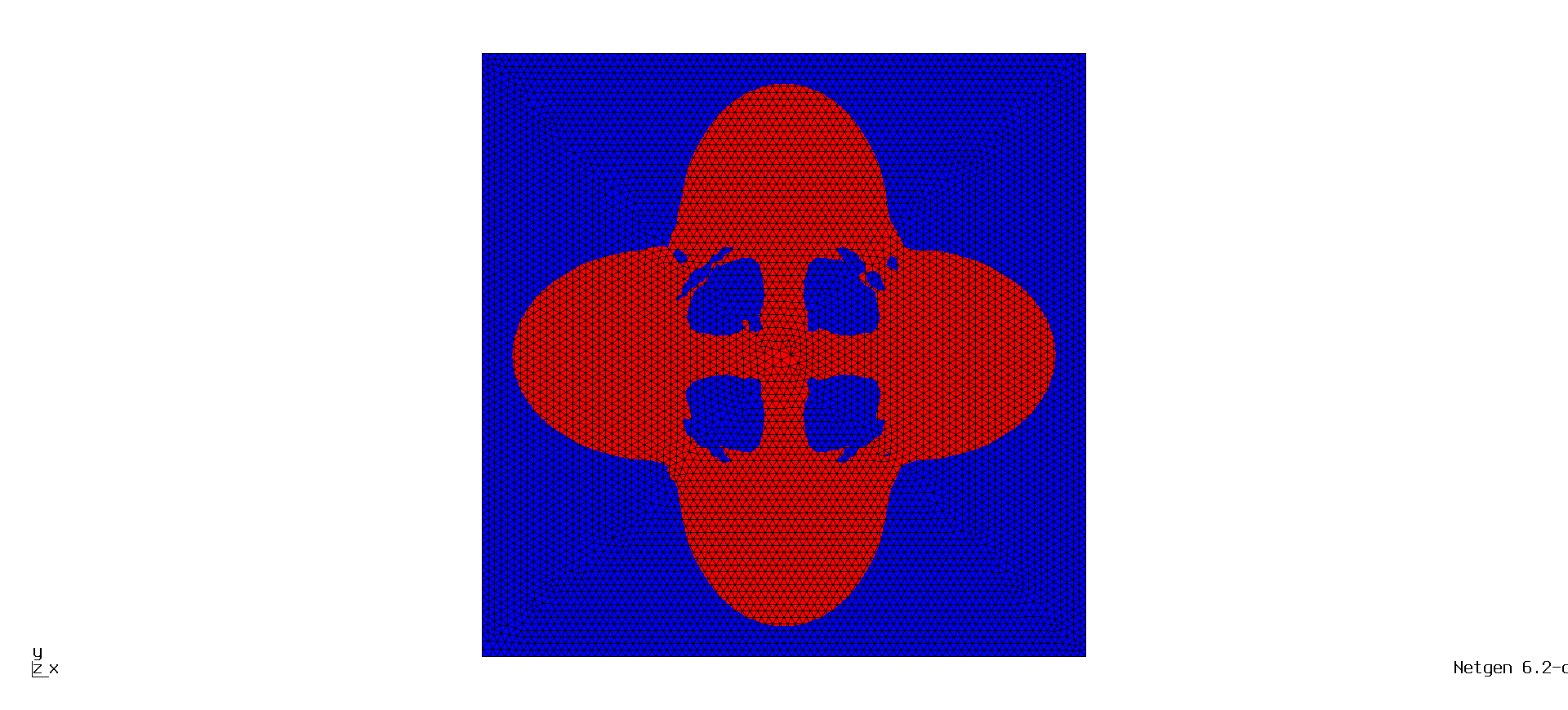
As an optimal shape we define \(\Omega_{opt} := \{f<0\}\), where \(f\) is the function from the levelset example describing a clover shape. We construct \(u_d\) by solving
[6]:
a = 4.0/5.0
b = 2
f = CoefficientFunction( 0.1*( (sqrt((x - a)**2 + b * y**2) - 1) \
                * (sqrt((x + a)**2 + b * y**2) - 1) \
                * (sqrt(b * x**2 + (y - a)**2) - 1) \
                * (sqrt(b * x**2 + (y + a)**2) - 1) - 0.001) )

psides.Set(f)
InterpolateLevelSetToElems(psides, beta1, beta2, beta, mesh, EPS)
InterpolateLevelSetToElems(psides, f1, f2, f_rhs, mesh, EPS)

B.Assemble()
L.Assemble()
inv = B.mat.Inverse(fes_state.FreeDofs(), inverse="sparsecholesky") # inverse of bilinear form

gfud.vec.data = inv*L.vec

Draw(gfud, mesh, 'gfud')
[6]:
BaseWebGuiScene
The function SolvePDE solves the state and adjoint state each time it is called. Note that since the functions beta and f_rhs are GridFunctions we do not have to re-define the bilinear form and linear form when beta and f_rhs change.
[7]:
def SolvePDE(adjoint=False):
    #Newton(a, gfu, printing = False, maxerr = 3e-9)

    B.Assemble()
    L.Assemble()

    inv_state = B.mat.Inverse(fes_state.FreeDofs(), inverse="sparsecholesky")

    # solve state equation
    gfu.vec.data = inv_state*L.vec

    if adjoint == True:
        # solve adjoint state equatoin
        duCost.Assemble()
        B_adj.Assemble()
        inv_adj = B_adj.mat.Inverse(fes_adj.FreeDofs(), inverse="sparsecholesky")
        gfp.vec.data = -inv_adj * duCost.vec
    scene_u.Redraw()

InterpolateLevelSetToElems(psi, beta1, beta2, beta, mesh, EPS)
InterpolateLevelSetToElems(psi, f1, f2, f_rhs, mesh, EPS)

SolvePDE()

# define the cost function
def Cost(u):
    return (u - gfud)**2*dx

# derivative of cost function
duCost += 2*(gfu-gfud) * q * dx

print("initial cost = ", Integrate(Cost(gfu), mesh))
initial cost = 39.29567644495133
It remains to implement the topological derivative: In define \(NegPos\) and \(PosNeg\) as the topological derivative in \(\Omega\) respectively \(D \setminus \overline{\Omega}\):
and the update function (also called generalised topological derivative)
[8]:
BetaPosNeg = 2 * beta2 * (beta1-beta2)/(beta1+beta2)    # factors in TD in positive part {x: \psi(x)>0} ={x: \beta(x) = \beta_2}
BetaNegPos = 2 * beta1 * (beta1-beta2)/(beta1+beta2)    # factors in TD in positive part {x: \psi(x)>0} ={x: \beta(x) = \beta_2}
FPosNeg = -(f1-f2)

psinew.vec.data = psi.vec

## normalise psi in L2
normPsi = sqrt(Integrate(psi**2*dx, mesh))
psi.vec.data = 1/normPsi * psi.vec

kappa = 0.05

# set level set function to data
InterpolateLevelSetToElems(psi, beta1, beta2, beta, mesh, EPS)
InterpolateLevelSetToElems(psi, f1, f2, f_rhs, mesh, EPS)

Redraw()

TD_node = GridFunction(fes_level)
#scene1 = Draw(TD_node, mesh, "TD_node")

TD_pwc = GridFunction(pwc)
#scene2 = Draw(TD_pwc, mesh, "TD_pwc")

TDPosNeg_pwc = GridFunction(pwc)
TDNegPos_pwc = GridFunction(pwc)

cutRatio = GridFunction(pwc)

# solve for current configuration
SolvePDE(adjoint=True)
- Finally we can define a loop defining the levelset update: :nbsphinx-math:`begin{align*}
psi_{k+1} = (1-s_k) frac{psi_k}{|\psi_k|} + s_k frac{g_{psi_k}}{|g_{\psi_k}|}
end{align*}`
[9]:
scene = Draw(psi)
scene_cr = Draw(cutRatio, mesh, "cutRatio")
[10]:
iter_max = 20
converged = False

xm=0.
ym=0.
psi.Set( (x-xm)**2+(y-ym)**2-0.25**2)
psinew.vec.data= psi.vec
scene.Redraw()

J = Integrate(Cost(gfu),mesh)

with TaskManager():

    for k in range(iter_max):
        print("================ iteration ", k, "===================")

        # copy new levelset data from psinew into psi
        psi.vec.data = psinew.vec
        scene.Redraw()


        SolvePDE(adjoint=True)

        J_current = Integrate(Cost(gfu),mesh)

        print( Integrate( (gfu-gfud)**2*dx, mesh) )

        print("cost in beginning of iteration", k, ": Cost = ", J_current)

        # compute the piecewise constant topological derivative in each domain
        TDPosNeg_pwc.Set( BetaPosNeg * grad(gfu) * grad(gfp)  + FPosNeg*gfp )
        TDNegPos_pwc.Set( BetaNegPos * grad(gfu) * grad(gfp)  + FPosNeg*gfp )

        # compute the cut ratio of the interface elements
        InterpolateLevelSetToElems(psi, 1, 0, cutRatio, mesh, EPS)
        scene_cr.Redraw()

        # compute the combined topological derivative using the cut ratio information
        for j in range(len(TD_pwc.vec)):
            TD_pwc.vec[j] = cutRatio.vec[j] * TDNegPos_pwc.vec[j] + (1-cutRatio.vec[j])*TDPosNeg_pwc.vec[j]

        TD_node.Set(TD_pwc)

        normTD = sqrt(Integrate(TD_node**2*dx, mesh)) # L2 norm of TD_node
        TD_node.vec.data = 1/normTD * TD_node.vec # normalised TD_node

        normPsi = sqrt(Integrate(psi**2*dx, mesh)) # L2 norm of psi
        psi.vec.data = 1/normPsi * psi.vec  # normalised psi

        linesearch = True

        for j in range(10):

            # update the level set function
            psinew.vec.data = (1-kappa)*psi.vec + kappa*TD_node.vec

            # update beta and f_rhs
            InterpolateLevelSetToElems(psinew, beta1, beta2, beta, mesh, EPS)
            InterpolateLevelSetToElems(psinew, f1, f2, f_rhs, mesh, EPS)

            # solve PDE without adjoint
            SolvePDE()

            Redraw(blocking=True)

            Jnew = Integrate(Cost(gfu), mesh)

            if Jnew > J_current:
                print("--------------------")
                print("-----line search ---")
                print("--------------------")
                kappa = kappa*0.8
                print("kappa", kappa)
            else:
                break

        Redraw(blocking=True)
        print("----------- Jnew in  iteration ", k, " = ", Jnew, " (kappa = ", kappa, ")")
        print('')
        print("iter" + str(k) + ", Jnew = " + str(Jnew) + " (kappa = ", kappa, ")")
        kappa = min(1, kappa*1.2)

        print("end of iter " + str(k))
================ iteration  0 ===================
39.295676444951326
cost in beginning of iteration 0 : Cost =  39.295676444951326
----------- Jnew in  iteration  0  =  11.859500825447777  (kappa =  0.05 )

iter0, Jnew = 11.859500825447777 (kappa =  0.05 )
end of iter 0
================ iteration  1 ===================
11.8595008254479
cost in beginning of iteration 1 : Cost =  11.859500825447899
----------- Jnew in  iteration  1  =  6.366217031113669  (kappa =  0.06 )

iter1, Jnew = 6.366217031113669 (kappa =  0.06 )
end of iter 1
================ iteration  2 ===================
6.366217031113584
cost in beginning of iteration 2 : Cost =  6.366217031113586
----------- Jnew in  iteration  2  =  6.219404002335032  (kappa =  0.072 )

iter2, Jnew = 6.219404002335032 (kappa =  0.072 )
end of iter 2
================ iteration  3 ===================
6.219404002335112
cost in beginning of iteration 3 : Cost =  6.2194040023351125
--------------------
-----line search ---
--------------------
kappa 0.06912
--------------------
-----line search ---
--------------------
kappa 0.055296000000000005
--------------------
-----line search ---
--------------------
kappa 0.04423680000000001
--------------------
-----line search ---
--------------------
kappa 0.03538944000000001
--------------------
-----line search ---
--------------------
kappa 0.028311552000000007
--------------------
-----line search ---
--------------------
kappa 0.02264924160000001
--------------------
-----line search ---
--------------------
kappa 0.018119393280000007
--------------------
-----line search ---
--------------------
kappa 0.014495514624000005
----------- Jnew in  iteration  3  =  5.650460303042802  (kappa =  0.014495514624000005 )

iter3, Jnew = 5.650460303042802 (kappa =  0.014495514624000005 )
end of iter 3
================ iteration  4 ===================
5.650460303042789
cost in beginning of iteration 4 : Cost =  5.650460303042789
--------------------
-----line search ---
--------------------
kappa 0.013915694039040007
----------- Jnew in  iteration  4  =  5.538240999806252  (kappa =  0.013915694039040007 )

iter4, Jnew = 5.538240999806252 (kappa =  0.013915694039040007 )
end of iter 4
================ iteration  5 ===================
5.538240999805482
cost in beginning of iteration 5 : Cost =  5.538240999805483
--------------------
-----line search ---
--------------------
kappa 0.013359066277478408
--------------------
-----line search ---
--------------------
kappa 0.010687253021982727
--------------------
-----line search ---
--------------------
kappa 0.008549802417586181
--------------------
-----line search ---
--------------------
kappa 0.006839841934068946
----------- Jnew in  iteration  5  =  5.477093516467158  (kappa =  0.006839841934068946 )

iter5, Jnew = 5.477093516467158 (kappa =  0.006839841934068946 )
end of iter 5
================ iteration  6 ===================
5.477093516467165
cost in beginning of iteration 6 : Cost =  5.477093516467165
--------------------
-----line search ---
--------------------
kappa 0.006566248256706188
----------- Jnew in  iteration  6  =  5.085963722546276  (kappa =  0.006566248256706188 )

iter6, Jnew = 5.085963722546276 (kappa =  0.006566248256706188 )
end of iter 6
================ iteration  7 ===================
5.0859637225464365
cost in beginning of iteration 7 : Cost =  5.0859637225464365
--------------------
-----line search ---
--------------------
kappa 0.00630359832643794
--------------------
-----line search ---
--------------------
kappa 0.005042878661150352
--------------------
-----line search ---
--------------------
kappa 0.004034302928920282
----------- Jnew in  iteration  7  =  5.024676369417681  (kappa =  0.004034302928920282 )

iter7, Jnew = 5.024676369417681 (kappa =  0.004034302928920282 )
end of iter 7
================ iteration  8 ===================
5.0246763694176915
cost in beginning of iteration 8 : Cost =  5.0246763694176915
--------------------
-----line search ---
--------------------
kappa 0.003872930811763471
----------- Jnew in  iteration  8  =  4.68016400292861  (kappa =  0.003872930811763471 )

iter8, Jnew = 4.68016400292861 (kappa =  0.003872930811763471 )
end of iter 8
================ iteration  9 ===================
4.680164002928659
cost in beginning of iteration 9 : Cost =  4.680164002928659
--------------------
-----line search ---
--------------------
kappa 0.003718013579292932
--------------------
-----line search ---
--------------------
kappa 0.0029744108634343455
--------------------
-----line search ---
--------------------
kappa 0.0023795286907474767
--------------------
-----line search ---
--------------------
kappa 0.0019036229525979814
----------- Jnew in  iteration  9  =  4.548013307503995  (kappa =  0.0019036229525979814 )

iter9, Jnew = 4.548013307503995 (kappa =  0.0019036229525979814 )
end of iter 9
================ iteration  10 ===================
4.548013307503997
cost in beginning of iteration 10 : Cost =  4.548013307503997
----------- Jnew in  iteration  10  =  4.297138500841579  (kappa =  0.0022843475431175778 )

iter10, Jnew = 4.297138500841579 (kappa =  0.0022843475431175778 )
end of iter 10
================ iteration  11 ===================
4.297138500841646
cost in beginning of iteration 11 : Cost =  4.297138500841644
--------------------
-----line search ---
--------------------
kappa 0.002192973641392875
--------------------
-----line search ---
--------------------
kappa 0.0017543789131143001
--------------------
-----line search ---
--------------------
kappa 0.00140350313049144
----------- Jnew in  iteration  11  =  4.240506681974793  (kappa =  0.00140350313049144 )

iter11, Jnew = 4.240506681974793 (kappa =  0.00140350313049144 )
end of iter 11
================ iteration  12 ===================
4.240506681974803
cost in beginning of iteration 12 : Cost =  4.240506681974803
----------- Jnew in  iteration  12  =  4.116140835707622  (kappa =  0.0016842037565897282 )

iter12, Jnew = 4.116140835707622 (kappa =  0.0016842037565897282 )
end of iter 12
================ iteration  13 ===================
4.116140835707513
cost in beginning of iteration 13 : Cost =  4.116140835707513
----------- Jnew in  iteration  13  =  4.1052025618857435  (kappa =  0.002021044507907674 )

iter13, Jnew = 4.1052025618857435 (kappa =  0.002021044507907674 )
end of iter 13
================ iteration  14 ===================
4.105202561885752
cost in beginning of iteration 14 : Cost =  4.105202561885752
----------- Jnew in  iteration  14  =  4.030283152749486  (kappa =  0.0024252534094892086 )

iter14, Jnew = 4.030283152749486 (kappa =  0.0024252534094892086 )
end of iter 14
================ iteration  15 ===================
4.030283152749549
cost in beginning of iteration 15 : Cost =  4.03028315274955
--------------------
-----line search ---
--------------------
kappa 0.00232824327310964
--------------------
-----line search ---
--------------------
kappa 0.0018625946184877122
----------- Jnew in  iteration  15  =  4.013358364173734  (kappa =  0.0018625946184877122 )

iter15, Jnew = 4.013358364173734 (kappa =  0.0018625946184877122 )
end of iter 15
================ iteration  16 ===================
4.013358364173748
cost in beginning of iteration 16 : Cost =  4.013358364173748
----------- Jnew in  iteration  16  =  3.884567520528918  (kappa =  0.0022351135421852545 )

iter16, Jnew = 3.884567520528918 (kappa =  0.0022351135421852545 )
end of iter 16
================ iteration  17 ===================
3.884567520528848
cost in beginning of iteration 17 : Cost =  3.884567520528848
--------------------
-----line search ---
--------------------
kappa 0.0021457090004978444
--------------------
-----line search ---
--------------------
kappa 0.0017165672003982757
----------- Jnew in  iteration  17  =  3.8369927695951387  (kappa =  0.0017165672003982757 )

iter17, Jnew = 3.8369927695951387 (kappa =  0.0017165672003982757 )
end of iter 17
================ iteration  18 ===================
3.8369927695951485
cost in beginning of iteration 18 : Cost =  3.8369927695951485
----------- Jnew in  iteration  18  =  3.7363831838099792  (kappa =  0.0020598806404779307 )

iter18, Jnew = 3.7363831838099792 (kappa =  0.0020598806404779307 )
end of iter 18
================ iteration  19 ===================
3.7363831838099473
cost in beginning of iteration 19 : Cost =  3.7363831838099473
--------------------
-----line search ---
--------------------
kappa 0.0019774854148588133
----------- Jnew in  iteration  19  =  3.7181392146687866  (kappa =  0.0019774854148588133 )

iter19, Jnew = 3.7181392146687866 (kappa =  0.0019774854148588133 )
end of iter 19
After 999 iterations: $J = $
[ ]: