This page was generated from unit-2.1.3-bddc/bddc.ipynb.
2.1.3 Element-wise BDDC Preconditioner
The element-wise BDDC (Balancing Domain Decomposition preconditioner with Constraints) preconditioner in NGSolve is a good general purpose preconditioner that works well both in the shared memory parallel mode as well as in distributed memory mode. In this tutorial, we discuss this preconditioner, related built-in options, and customization from python.
Let us start with a simple description of the element-wise BDDC in the context of Lagrange finite element space \(V\). Here the BDDC preconditoner is constructed on an auxiliary space \(\widetilde{V}\) obtained by connecting only element vertices (leaving edge and face shape functions discontinuous). Although larger, the auxiliary space allows local elimination of edge and face variables. Hence an analogue of the original matrix \(A\) on this space, named \(\widetilde A\), is less expensive to invert. This inverse is used to construct a preconditioner for \(A\) as follows:
Here, \(R\) is the averaging operator for the discontinous edge and face variables.
To construct a general purpose BDDC preconditioner, NGSolve generalizes this idea to all its finite element spaces by a classification of degrees of freedom. Dofs are classified into (condensable) LOCAL_DOFs that we saw in 1.4 and a remainder that includes these types:
WIREBASKET_DOFINTERFACE_DOFThe original finite element space \(V\) is obtained by requiring conformity of both the above types of dofs, while the auxiliary space \(\widetilde{V}\) is obtained by requiring conformity of WIREBASKET_DOFs only.
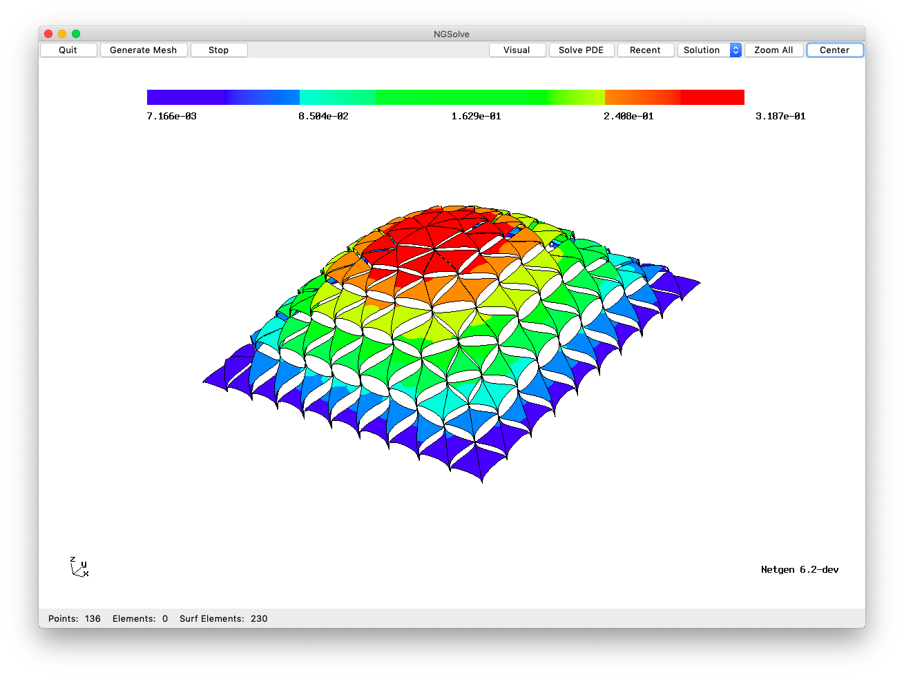
Here is a figure of a typical function in the default \(\widetilde{V}\) (and the code to generate this is at the end of this tutorial) when \(V\) is the Lagrange space:
[1]:
from ngsolve import *
from ngsolve.webgui import Draw
from ngsolve.la import EigenValues_Preconditioner
from netgen.csg import unit_cube
from netgen.geom2d import unit_square
SetHeapSize(100*1000*1000)
[2]:
mesh = Mesh(unit_cube.GenerateMesh(maxh=0.5))
# mesh = Mesh(unit_square.GenerateMesh(maxh=0.5))
Built-in options
Let us define a simple function to study how the spectrum of the preconditioned matrix changes with various options.
Effect of condensation
[3]:
def TestPreconditioner (p, condense=False, **args):
    fes = H1(mesh, order=p, **args)
    u,v = fes.TnT()
    a = BilinearForm(fes, eliminate_internal=condense)
    a += grad(u)*grad(v)*dx + u*v*dx
    c = Preconditioner(a, "bddc")
    a.Assemble()
    return EigenValues_Preconditioner(a.mat, c.mat)
[4]:
lams = TestPreconditioner(5)
print (lams[0:3], "...\n", lams[-3:])
 1.00234
 1.04127
 1.13435
 ...
  7.40944
 7.63426
 7.66348
Here is the effect of static condensation on the BDDC preconditioner.
[5]:
lams = TestPreconditioner(5, condense=True)
print (lams[0:3], "...\n", lams[-3:])
 1.00142
 1.03925
   1.115
 ...
  6.92373
 7.01755
 7.29845
Tuning the auxiliary space
Next, let us study the effect of a few built-in flags for finite element spaces that are useful for tweaking the behavior of the BDDC preconditioner. The effect of these flags varies in two (2D) and three dimensions (3D), e.g.,
wb_fulledges=True: This option keeps all edge-dofs conforming (i.e. they are markedWIREBASKET_DOFs). This option is only meaningful in 3D. If used in 2D, the preconditioner becomes a direct solver.wb_withedges=True: This option keeps only the first edge-dof conforming (i.e., the first edge-dof is markedWIREBASKET_DOFand the remaining edge-dofs are markedINTERFACE_DOFs).
The complete situation is a bit more complex due to the fact these options can take the three values True, False, or Undefined, the two options can be combined, and the space dimension can be 2 or 3. The default value of these flags in NGSolve is Undefined. Here is a table with the summary of the effect of these options:
wb_fulledges |
wb_withedges |
2D |
3D |
|---|---|---|---|
True |
any value |
all |
all |
False/Undefined |
Undefined |
none |
first |
False/Undefined |
False |
none |
none |
False/Undefined |
True |
first |
first |
An entry \(X \in\) {all, none, first} of the last two columns is to be read as follows: \(X\) of the edge-dofs is(are) WIREBASKET_DOF(s).
Here is an example of the effect of one of these flag values.
[6]:
lams = TestPreconditioner(5, condense=True,
                          wb_withedges=False)
print (lams[0:3], "...\n", lams[-3:])
 1.00424
 1.09252
  1.3257
 ...
  31.0804
 33.0369
 33.6461
Clearly, when moving from the default case (where the first of the edge dofs are wire basket dofs) to the case (where none of the edge dofs are wire basket dofs), the conditioning became less favorable.
Customize
From within python, we can change the types of degrees of freedom of finite element spaces, thus affecting the behavior of the BDDC preconditioner.
To depart from the default and commit the first two edge dofs to wire basket, we perform the next steps:
[7]:
fes = H1(mesh, order=10)
u,v = fes.TnT()

for ed in mesh.edges:
    dofs = fes.GetDofNrs(ed)
    for d in dofs:
        fes.SetCouplingType(d, COUPLING_TYPE.INTERFACE_DOF)

    # Set the first two edge dofs to be conforming
    fes.SetCouplingType(dofs[0], COUPLING_TYPE.WIREBASKET_DOF)
    fes.SetCouplingType(dofs[1], COUPLING_TYPE.WIREBASKET_DOF)

a = BilinearForm(fes, eliminate_internal=True)
a += grad(u)*grad(v)*dx + u*v*dx
c = Preconditioner(a, "bddc")
a.Assemble()

lams=EigenValues_Preconditioner(a.mat, c.mat)
max(lams)/min(lams)
[7]:
18.179082265714545
This is a slight improvement from the default.
[8]:
lams = TestPreconditioner (10, condense=True)
max(lams)/min(lams)
[8]:
27.364417060939882
Combine BDDC with AMG for large problems
coarsetype=h1amg flag, we can ask BDDC to replace \({\,\widetilde{A}\,}^{-1}\) by an Algebraic MultiGrid (AMG) preconditioner. Since NGSolve’s h1amg is well-suitedwb_withedges=False to ensure that \(\widetilde{A}\) is made solely with vertex unknowns.[9]:
p = 5
mesh = Mesh(unit_cube.GenerateMesh(maxh=0.05))
fes = H1(mesh, order=p, dirichlet="left|bottom|back",
         wb_withedges=False)
print("NDOF = ", fes.ndof)
u,v = fes.TnT()
a = BilinearForm(fes)
a += grad(u)*grad(v)*dx
f = LinearForm(fes)
f += v*dx

with TaskManager():
    pre = Preconditioner(a, "bddc", coarsetype="h1amg")
    a.Assemble()
    f.Assemble()

    gfu = GridFunction(fes)
    solvers.CG(mat=a.mat, rhs=f.vec, sol=gfu.vec,
               pre=pre, maxsteps=500)
Draw(gfu)
NDOF =  1170736
WARNING: maxsteps is deprecated, use maxiter instead!
CG iteration 1, residual = 0.7094090868385201
CG iteration 2, residual = 0.27709235419647266
CG iteration 3, residual = 0.2552141476493644
CG iteration 4, residual = 0.29760250572557956
CG iteration 5, residual = 0.2551534050645899
CG iteration 6, residual = 0.19409338025273246
CG iteration 7, residual = 0.14466456735602168
CG iteration 8, residual = 0.1121652511855541
CG iteration 9, residual = 0.07951672978661896
CG iteration 10, residual = 0.05885836872647854
CG iteration 11, residual = 0.04343213200102174
CG iteration 12, residual = 0.035760102280393745
CG iteration 13, residual = 0.029804921900339107
CG iteration 14, residual = 0.021364235775509822
CG iteration 15, residual = 0.01639501848202992
CG iteration 16, residual = 0.013065067451515212
CG iteration 17, residual = 0.010281475047778653
CG iteration 18, residual = 0.007516183238695055
CG iteration 19, residual = 0.00540059910416029
CG iteration 20, residual = 0.004159975246836044
CG iteration 21, residual = 0.0033356715080478452
CG iteration 22, residual = 0.0025567178563386454
CG iteration 23, residual = 0.0018863277812046853
CG iteration 24, residual = 0.0014480171690318246
CG iteration 25, residual = 0.0011583796766805826
CG iteration 26, residual = 0.000906648118779185
CG iteration 27, residual = 0.0006879506314201755
CG iteration 28, residual = 0.0005269442608123831
CG iteration 29, residual = 0.00040115927332543406
CG iteration 30, residual = 0.00031503500823442244
CG iteration 31, residual = 0.0002498998602943324
CG iteration 32, residual = 0.00019082947428133447
CG iteration 33, residual = 0.00014315141755483858
CG iteration 34, residual = 0.00011174356552301843
CG iteration 35, residual = 8.567914626339037e-05
CG iteration 36, residual = 6.622157865058174e-05
CG iteration 37, residual = 5.077678888471282e-05
CG iteration 38, residual = 3.9347393964067066e-05
CG iteration 39, residual = 3.069965593023224e-05
CG iteration 40, residual = 2.33296313465556e-05
CG iteration 41, residual = 1.810177895187837e-05
CG iteration 42, residual = 1.4422937256375226e-05
CG iteration 43, residual = 1.1280700987011004e-05
CG iteration 44, residual = 8.67624883991304e-06
CG iteration 45, residual = 6.472767303048754e-06
CG iteration 46, residual = 5.003440601466716e-06
CG iteration 47, residual = 3.8283886709572356e-06
CG iteration 48, residual = 2.928339674985159e-06
CG iteration 49, residual = 2.2656179101176032e-06
CG iteration 50, residual = 1.8273692600402321e-06
CG iteration 51, residual = 1.4226184082012478e-06
CG iteration 52, residual = 1.0818334558222376e-06
CG iteration 53, residual = 8.099502945603018e-07
CG iteration 54, residual = 6.094730740744591e-07
CG iteration 55, residual = 4.6194864798528725e-07
CG iteration 56, residual = 3.5712097827880107e-07
CG iteration 57, residual = 2.7591527031657427e-07
CG iteration 58, residual = 2.182412897552225e-07
CG iteration 59, residual = 1.7485809206654927e-07
CG iteration 60, residual = 1.343199060404743e-07
CG iteration 61, residual = 1.007739734770355e-07
CG iteration 62, residual = 7.59258930665662e-08
CG iteration 63, residual = 5.952078091484163e-08
CG iteration 64, residual = 4.486106702868246e-08
CG iteration 65, residual = 3.4204272871611554e-08
CG iteration 66, residual = 2.6109240627975857e-08
CG iteration 67, residual = 1.9906599352017872e-08
CG iteration 68, residual = 1.5466948940628753e-08
CG iteration 69, residual = 1.1695566290270323e-08
CG iteration 70, residual = 8.963548384249897e-09
CG iteration 71, residual = 6.810820217694138e-09
CG iteration 72, residual = 5.212600493113718e-09
CG iteration 73, residual = 3.9848212511377645e-09
CG iteration 74, residual = 3.022515412039782e-09
CG iteration 75, residual = 2.299369047374858e-09
CG iteration 76, residual = 1.7707357241093148e-09
CG iteration 77, residual = 1.3495559498594945e-09
CG iteration 78, residual = 1.0254808766559746e-09
CG iteration 79, residual = 7.813150725795362e-10
CG iteration 80, residual = 6.029347132676393e-10
CG iteration 81, residual = 4.5959071718153433e-10
CG iteration 82, residual = 3.4385966777049143e-10
CG iteration 83, residual = 2.6570314996823507e-10
CG iteration 84, residual = 2.0308130752494843e-10
CG iteration 85, residual = 1.5554929001852785e-10
CG iteration 86, residual = 1.1872192316452685e-10
CG iteration 87, residual = 9.497264860417181e-11
CG iteration 88, residual = 7.640118648309322e-11
CG iteration 89, residual = 5.894390293345089e-11
CG iteration 90, residual = 4.4524744379412616e-11
CG iteration 91, residual = 3.403466400609331e-11
CG iteration 92, residual = 2.565921442614409e-11
CG iteration 93, residual = 1.9752977977492154e-11
CG iteration 94, residual = 1.5010944915581735e-11
CG iteration 95, residual = 1.125469896491788e-11
CG iteration 96, residual = 8.697092386480894e-12
CG iteration 97, residual = 6.646106274432163e-12
CG iteration 98, residual = 5.067916114206671e-12
CG iteration 99, residual = 3.791040961095745e-12
CG iteration 100, residual = 2.8942484397130418e-12
CG iteration 101, residual = 2.209252707852319e-12
CG iteration 102, residual = 1.674765825975621e-12
CG iteration 103, residual = 1.2810904118679393e-12
CG iteration 104, residual = 9.795089411054082e-13
CG iteration 105, residual = 7.569465754398145e-13
CG iteration 106, residual = 5.879722620166115e-13
[9]:
BaseWebGuiScene
Postscript
By popular demand, here is the code to draw the figure found at the beginning of this tutorial:
[10]:
from netgen.geom2d import unit_square
mesh = Mesh(unit_square.GenerateMesh(maxh=0.1))
fes_ho = Discontinuous(H1(mesh, order=10))
fes_lo = H1(mesh, order=1, dirichlet=".*")
fes_lam = Discontinuous(H1(mesh, order=1))
fes = FESpace([fes_ho, fes_lo, fes_lam])
uho, ulo, lam = fes.TrialFunction()

a = BilinearForm(fes)
a += Variation(0.5 * grad(uho)*grad(uho)*dx
               - 1*uho*dx
               + (uho-ulo)*lam*dx(element_vb=BBND))
gfu = GridFunction(fes)
solvers.Newton(a=a, u=gfu)
Draw(gfu.components[0],deformation=True)
Newton iteration  0
err =  0.39392955469293095
Newton iteration  1
err =  1.7898870223932246e-15
[10]:
BaseWebGuiScene
[ ]: