Navier Stokes Equation
We solve the time-dependent incompressible Navier Stokes Equation. For that
- we use the P3/P2 Taylor-Hood mixed finite element pairing
- and perform operator splitting time-integration with the non-linear term explicit, but time-dependent Stokes fully implicit.
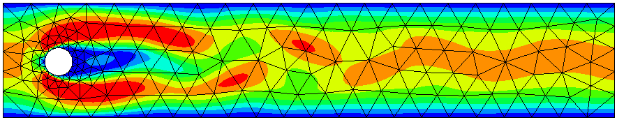
The example is from the Schäfer-Turek benchmark <http://www.mathematik.tu-dortmund.de/lsiii/cms/papers/SchaeferTurek1996.pdf> a two-dimensional cylinder, at Reynolds number 100
Download navierstokes.py
from ngsolve import *

# viscosity
nu = 0.001

# timestepping parameters
tau = 0.001
tend = 10

# mesh = Mesh("cylinder.vol")
from netgen.geom2d import SplineGeometry
geo = SplineGeometry()
geo.AddRectangle( (0, 0), (2, 0.41), bcs = ("wall", "outlet", "wall", "inlet"))
geo.AddCircle ( (0.2, 0.2), r=0.05, leftdomain=0, rightdomain=1, bc="cyl")
mesh = Mesh( geo.GenerateMesh(maxh=0.08))

mesh.Curve(3)

V = H1(mesh,order=3, dirichlet="wall|cyl|inlet")
Q = H1(mesh,order=2)

X = FESpace([V,V,Q])

ux,uy,p = X.TrialFunction()
vx,vy,q = X.TestFunction()

div_u = grad(ux)[0]+grad(uy)[1]
div_v = grad(vx)[0]+grad(vy)[1]

stokes = nu*grad(ux)*grad(vx)+nu*grad(uy)*grad(vy)+div_u*q+div_v*p - 1e-10*p*q
a = BilinearForm(X)
a += SymbolicBFI(stokes)
a.Assemble()

# nothing here ...
f = LinearForm(X)
f.Assemble()

# gridfunction for the solution
gfu = GridFunction(X)

# parabolic inflow at bc=1:
uin = 1.5*4*y*(0.41-y)/(0.41*0.41)
gfu.components[0].Set(uin, definedon=mesh.Boundaries("inlet"))

# solve Stokes problem for initial conditions:
inv_stokes = a.mat.Inverse(X.FreeDofs())

res = f.vec.CreateVector()
res.data = f.vec - a.mat*gfu.vec
gfu.vec.data += inv_stokes * res


# matrix for implicit Euler
mstar = BilinearForm(X)
mstar += SymbolicBFI(ux*vx+uy*vy + tau*stokes)
mstar.Assemble()
inv = mstar.mat.Inverse(X.FreeDofs(), inverse="sparsecholesky")

# the non-linear term
conv = BilinearForm(X, flags = { "nonassemble" : True })
conv += SymbolicBFI( CoefficientFunction( (ux,uy) ) * (grad(ux)*vx+grad(uy)*vy) )

# for visualization
velocity = CoefficientFunction (gfu.components[0:2])
Draw (Norm(velocity), mesh, "velocity", sd=3)

# implicit Euler/explicit Euler splitting method:
t = 0
with TaskManager():
    while t < tend:
        print ("t=", t)

        conv.Apply (gfu.vec, res)
        res.data += a.mat*gfu.vec
        gfu.vec.data -= tau * inv * res

        t = t + tau
        Redraw()
The absolute value of velocity: