This page was generated from unit-11.4-vie-Helmholtz/LippmannSchwinger.ipynb.

11.4.1 Lippmann-Schwinger equation

keys: volume integral equation, volume potential, penetrable scatterer, Mie series, Luneburg lens

from netgen.occ import *
from ngsolve import *
from ngsolve.webgui import Draw
from ngsolve.bem import *
from ngsolve.krylovspace import GMRESSolver
import numpy as np
import matplotlib.pyplot as plt
from scipy.special import spherical_jn, spherical_yn

dxi = dx(bonus_intorder=2)

Scattering by a penetrable sphere

The total field \(u = u_{in} + u_s\), with incoming wave \(u_{in} = e^{ikz}\) and outgoing scattered field \(u_s\), solves

\[\Delta u + k^2 \eta(x)^2 \, u = 0 \qquad \text{in} \, \mathbb R^3,\]

where the refractive index \(\eta\), the ratio of the outside to the local wave speed, equals 1 outside the scatterer \(D\). Moving the material to the right hand side and subtracting \((\Delta + k^2) u_{in} = 0\) gives, with the contrast \(m = 1-\eta^2\),

\[(\Delta + k^2) \, u_s = k^2 (1-\eta^2) \, u = k^2 m u.\]

The material acts as a source that vanishes outside \(D\). Green’s representation formula for the outgoing field \(u_s\) gives \(u_s = -V_k\big((\Delta + k^2)\,u_s\big) = -k^2 V_k(m u)\), and adding \(u_{in}\) gives the Lippmann-Schwinger equation

\[u + k^2 \, V_k(m u) = u_{in} \qquad \text{in} \, D.\]

We multiply by a test function \(v\), integrate over \(D\), and solve for \(u_h\)

\[(u_h, v) + k^2 \big( V_k(m u_h), v \big) = (u_{in}, v) \qquad \forall \, v\]

where \((\cdot, \cdot)\) denotes the integral over \(D\)

def SolveLS(mesh, m, k, order):
    fes = L2(mesh, order=order, complex=True)
    u,v = fes.TnT()
    with TaskManager():
        M = BilinearForm(u*v*dx).Assemble()
        V = HelmholtzSL(m*u*dxi, k)*v*dxi
        rhs = LinearForm(exp(1j*k*z)*v*dxi).Assemble()
        inv = GMRESSolver(M.mat + k**2*V.mat, M.mat.Inverse(), tol=1e-8)
        gfu = GridFunction(fes)
        gfu.vec.data = inv * rhs.vec
    return gfu, inv.iterations

Once \(u_h\) is known, \(u_s = -k^2 V_k(m u_h)\) can be evaluated anywhere, also inside \(D\). We use the square \([-3,3]^2\) in the \(xz\)-plane.

plane = WorkPlane(Axes((0,0,0), n=Y, h=X)).RectangleC(6,6).Face()
disk = WorkPlane(Axes((0,0,0), n=Y, h=X)).Circle(0,0,1).Face()
pmesh = Mesh(OCCGeometry(Glue([plane-disk, disk])).GenerateMesh(maxh=0.2))
screen = pmesh.Boundaries(".*")

def ScatteredField(gfu, m, k):
    u = gfu.space.TrialFunction()
    return -k**2*HelmholtzSL(m*u*dxi, k)(gfu, screen)

For the unit sphere with constant \(\eta\), the Mie series is the exact solution. With \(k_1 = k \eta\),

\[u = \sum_l i^l (2l+1) \, a_l \, j_l(k_1 r) \, P_l(\cos \theta) \quad \text{in} \, D, \qquad u_s = \sum_l i^l (2l+1) \, b_l \, h^{(1)}_l(k r) \, P_l(\cos \theta) \quad \text{outside},\]

where \(a_l, b_l\) follow from the continuity of \(u\) and \(\partial_r u\) at \(r = 1\).

def Mie(k, eta):
    k1 = k*eta
    l = np.arange(int(k1)+16)
    j, dj = spherical_jn(l, k), spherical_jn(l, k, True)
    h, dh = j+1j*spherical_yn(l, k), dj+1j*spherical_yn(l, k, True)
    j1, dj1 = spherical_jn(l, k1), spherical_jn(l, k1, True)
    b = (k1*dj1*j-k*dj*j1) / (k*dh*j1-k1*dj1*h)
    return l, (j+b*h)/j1, b, k1

def MieOnAxis(k, eta, zs):
    l, a, b, k1 = Mie(k, eta)
    r, c = abs(zs)[:,None], 1j**l*(2*l+1)*np.where(zs < 0, -1, 1)[:,None]**l
    i, o = abs(zs) < 1, abs(zs) >= 1
    u = np.exp(1j*k*zs)
    u[i] = (c[i]*a*spherical_jn(l, k1*r[i])).sum(axis=1)
    u[o] += (c[o]*b*(spherical_jn(l, k*r[o])+1j*spherical_yn(l, k*r[o]))).sum(axis=1)
    return u

k, eta = 2, sqrt(2)
m = 1-eta**2
zs = np.linspace(-3, 3, 300)
zaxis = pmesh(0*zs, 0*zs, zs, BND)
inner = abs(zs) < 0.95
zin = zs[inner]
uz_mie = MieOnAxis(k, eta, zs)
err = lambda u, uex: np.linalg.norm(u-uex) / np.linalg.norm(uex)

cases = [(0.3, 0), (0.2, 0), (0.3, 1)]
print (" maxh  order  ndof  its  u_in+u_s   u_h")
uzs = []
for h, order in cases:
    mesh = Mesh(OCCGeometry(Sphere((0,0,0), 1)).GenerateMesh(maxh=h)).Curve(2)
    gfu, its = SolveLS(mesh, m, k, order)
    with TaskManager():
        uz = np.exp(1j*k*zs) + ScatteredField(gfu, m, k)(zaxis)[:,0]
    uzs.append(uz)
    uh = gfu(mesh(0*zin, 0*zin, zin))[:,0]
    print (f" {h:4.2f}  {order:5d}  {gfu.space.ndof:4d}  {its:3d}  "
           f"{err(uz[inner], uz_mie[inner]):.2e}  {err(uh, uz_mie[inner]):.2e}")

 maxh  order  ndof  its  u_in+u_s   u_h
 0.30      0   422   12  7.40e-02  3.60e-01
 0.20      0  1709   11  1.63e-02  1.17e-01
 0.30      1  1688   11  3.92e-03  6.77e-02

plt.plot(zs, uz_mie.real, "k", label="Mie")
for (h, order), uz in zip(cases, uzs):
    plt.plot(zs, uz.real, "--", label=f"maxh={h}, order={order}")
plt.axvspan(-1, 1, color="0.9"); plt.xlabel("$z$"); plt.ylabel("Re $u$"); plt.legend();

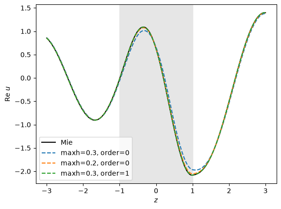
The table compares, for \(k = 2\) and \(\eta = \sqrt 2\), the total field \(u_{in} + u_s\) and \(u_h\) itself with the Mie series on the \(z\)-axis inside \(D\). Total field on the plane:

uscat = GridFunction(H1(pmesh, order=3, complex=True))
with TaskManager():
    uscat.Set(ScatteredField(gfu, m, k), definedon=screen)
Draw (exp(1j*k*z)+uscat, pmesh, min=-2, max=2, animate_complex=True, order=3, euler_angles=[90,0,0]);

Variable index: Luneburg lens

The Luneburg lens is a sphere with refractive index \(\eta = \sqrt{2 - r^2}\): the index decreases from \(\sqrt 2\) at the center to 1 at the surface, so it matches the surrounding medium without a jump. In the ray-optics limit, the rays of an incoming plane wave are bent inside the sphere and all meet in one point on the opposite side. At \(k = 5\) the wavelength \(2\pi/5 \approx 1.26\) is comparable to the radius, and the focus is inside the sphere near \(z \approx 0.8\). For larger \(k\) it moves toward \(z = 1\). SolveLS is reused unchanged, now with \(k = 5\) and the coefficient function \(m = 1 - \eta^2 = r^2 - 1\) as contrast:

k = 5
m = x**2+y**2+z**2-1
mesh = Mesh(OCCGeometry(Sphere((0,0,0), 1)).GenerateMesh(maxh=0.25)).Curve(2)
gfu, its = SolveLS(mesh, m, k, order=1)
print ("ndof =", gfu.space.ndof, ", GMRES iterations:", its)

ndof = 3936 , GMRES iterations: 18

with TaskManager():
    uscat.Set(ScatteredField(gfu, m, k), definedon=screen)
Draw(exp(1j*k*z)+uscat, pmesh, animate_complex=True, order=3, euler_angles=[90,0,0]);
ulens = abs(np.exp(1j*k*zs) + uscat(zaxis)[:,0])
print ("max |u| =", ulens.max(), "at z =", zs[ulens.argmax()])

max |u| = 3.380945976614123 at z = 0.8127090301003346