This page was generated from unit-1.6-adaptivity/adaptivity.ipynb.
1.6 Error estimation & adaptive refinement
In this tutorial, we apply a Zienkiewicz-Zhu type error estimator and run an adaptive loop with these steps:
[1]:
from ngsolve import *
from ngsolve.webgui import Draw
from netgen.occ import *
import matplotlib.pyplot as plt
Geometry
The following geometry represents a heated chip embedded in another material that conducts away the heat.
[2]:
def MakeGeometryOCC():
    base = Rectangle(1, 0.6).Face()
    chip = MoveTo(0.5,0.15).Line(0.15,0.15).Line(-0.15,0.15).Line(-0.15,-0.15).Close().Face()
    top = MoveTo(0.2,0.6).Rectangle(0.6,0.2).Face()
    base -= chip

    base.faces.name="base"
    chip.faces.name="chip"
    chip.faces.col=(1,0,0)
    top.faces.name="top"
    geo = Glue([base,chip,top])
    geo.edges.name="default"
    geo.edges.Min(Y).name="bot"
    return OCCGeometry(geo, dim=2)

mesh = Mesh(MakeGeometryOCC().GenerateMesh(maxh=0.2))
Draw(mesh)
[2]:
BaseWebGuiScene
Spaces & forms
The problem is to find \(u\) in \(H_{0,D}^1\) satisfying
for all \(v\) in \(H_{0,D}^1\). We expect the solution to have singularities due to the nonconvex re-enrant angles and discontinuities in \(\lambda\).
[3]:
fes = H1(mesh, order=3, dirichlet=[1])
u, v = fes.TnT()

# one heat conductivity coefficient per sub-domain
lam = CoefficientFunction([1, 1000, 10])
a = BilinearForm(lam*grad(u)*grad(v)*dx)

# heat-source in inner subdomain
f = LinearForm(fes)
f = LinearForm(1*v*dx(definedon="chip"))

c = Preconditioner(a, type="multigrid", inverse="sparsecholesky")

gfu = GridFunction(fes)
Note that the linear system is not yet assembled above.
Solve
Since we must solve multiple times, we define a function to solve the boundary value problem, where assembly, update, and solve occurs.
[4]:
def SolveBVP():
    fes.Update()
    gfu.Update()
    a.Assemble()
    f.Assemble()
    inv = CGSolver(a.mat, c.mat)
    gfu.vec.data = inv * f.vec
[5]:
SolveBVP()
Draw(gfu);
Estimate
We implement a gradient-recovery-type error estimator. For this, we need an H(div) space for flux recovery. We must compute the flux of the computed solution and interpolate it into this H(div) space.
[6]:
space_flux = HDiv(mesh, order=2)
gf_flux = GridFunction(space_flux, "flux")

flux = lam * grad(gfu)
gf_flux.Set(flux)
Element-wise error estimator: On each element \(T\), set
where \(u_h\) is the computed solution gfu and \(I_h\) is the interpolation performed by Set in NGSolve.
[7]:
err = 1/lam*(flux-gf_flux)*(flux-gf_flux)
Draw(err, mesh, 'error_representation')
[7]:
BaseWebGuiScene
[8]:
eta2 = Integrate(err, mesh, VOL, element_wise=True)
print(eta2)
 6.68417e-10
 7.62254e-08
 8.65452e-06
 5.00116e-10
 8.8811e-08
 5.49489e-09
 3.02529e-07
 7.32725e-10
 1.12641e-08
 2.98627e-08
 1.04189e-07
 2.50948e-07
 7.0518e-08
 8.00722e-07
 7.60703e-06
 9.7881e-07
 7.00995e-08
 7.58091e-06
 2.03482e-06
 2.44616e-08
 1.60629e-07
 6.52305e-08
 1.65889e-06
 1.15213e-06
 3.48558e-07
 2.50622e-06
 1.38426e-09
 1.80477e-06
 1.12638e-06
 4.9493e-08
 1.55159e-07
 1.58315e-09
 1.90147e-08
 1.92754e-08
 1.1525e-09
 9.74872e-10
 6.82708e-09
 8.52244e-10
 1.43383e-10
 9.7114e-09
The above values, one per element, lead us to identify elements which might have large error.
Mark
We mark elements with large error estimator for refinement.
[9]:
maxerr = max(eta2)
print ("maxerr = ", maxerr)

for el in mesh.Elements():
    mesh.SetRefinementFlag(el, eta2[el.nr] > 0.25*maxerr)
    # see below for vectorized alternative
maxerr = 8.654516606473739e-06
Refine & solve again
Refine marked elements:
[10]:
mesh.Refine()
SolveBVP()
Draw(gfu)
[10]:
BaseWebGuiScene
Automate the above steps
[11]:
l = []    # l = list of estimated total error

def CalcError():

    # compute the flux:
    space_flux.Update()
    gf_flux.Update()
    flux = lam * grad(gfu)
    gf_flux.Set(flux)

    # compute estimator:
    err = 1/lam*(flux-gf_flux)*(flux-gf_flux)
    eta2 = Integrate(err, mesh, VOL, element_wise=True)
    maxerr = max(eta2)
    l.append ((fes.ndof, sqrt(sum(eta2))))
    print("ndof =", fes.ndof, " maxerr =", maxerr)

    # mark for refinement (vectorized alternative)
    mesh.ngmesh.Elements2D().NumPy()["refine"] = eta2.NumPy() > 0.25*maxerr
[12]:
CalcError()
mesh.Refine()
ndof = 355 maxerr = 5.091895627858535e-06
Run the adaptive loop
[13]:
level = 0
while fes.ndof < 50000:
    SolveBVP()
    level = level + 1
    if level%5 == 0:
        print('adaptive step #', level)
        Draw(gfu)
    CalcError()
    mesh.Refine()
ndof = 610  maxerr = 2.0453848565311223e-06
ndof = 1057  maxerr = 8.12039255699178e-07
ndof = 1498  maxerr = 3.2215379259212e-07
ndof = 2176  maxerr = 1.2779488709494257e-07
adaptive step # 5
ndof = 2977  maxerr = 5.0678146234551165e-08
ndof = 3895  maxerr = 2.0093310174656036e-08
ndof = 4711  maxerr = 8.091450961745783e-09
ndof = 5509  maxerr = 3.867954263623651e-09
ndof = 6271  maxerr = 1.8531027594497268e-09
adaptive step # 10
ndof = 6934  maxerr = 8.88873035130047e-10
ndof = 7678  maxerr = 4.266427654407609e-10
ndof = 8611  maxerr = 2.04847394308994e-10
ndof = 9745  maxerr = 9.837170261932882e-11
ndof = 10642  maxerr = 4.7244686455135854e-11
adaptive step # 15
ndof = 12292  maxerr = 2.2691238346581638e-11
ndof = 13735  maxerr = 1.0898484736138015e-11
ndof = 15721  maxerr = 5.23462725382843e-12
ndof = 17944  maxerr = 2.5142372957297096e-12
ndof = 20470  maxerr = 1.2076188731821963e-12
adaptive step # 20
ndof = 23848  maxerr = 5.800220063060348e-13
ndof = 27451  maxerr = 2.785973414967979e-13
ndof = 32353  maxerr = 1.3380949493027622e-13
ndof = 38077  maxerr = 6.427239229010473e-14
ndof = 43858  maxerr = 3.086943972821151e-14
adaptive step # 25
ndof = 51115 maxerr = 1.4827488819774688e-14
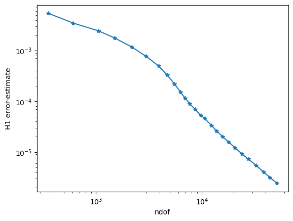
Plot history of adaptive convergence
[14]:
plt.yscale('log')
plt.xscale('log')
plt.xlabel("ndof")
plt.ylabel("H1 error-estimate")
ndof,err = zip(*l)
plt.plot(ndof,err, "-*")

plt.ion()
plt.show()