This page was generated from unit-6.1.3-rmplate/Reissner_Mindlin_plate.ipynb.

6.1.3 Reissner-Mindlin plate

To avoid shear locking when the thickness $t$ becomes small several methods and elements have been proposed. We discuss two approaches:

1: Mixed Interpolation of Tensorial Components (MITC)

2: Rotations in Nèdèlec space using the Tangential-Displacement Normal-Normal-Stress method (TDNNS)

Mixed Interpolation of Tensorial Components (MITC)

from ngsolve import *
from netgen.geom2d import SplineGeometry
from ngsolve.webgui import Draw

Set up benchmark example with exact solution. Young modulus $E$, Poisson ratio $\nu$, shear correction factor $\kappa$ and corresponding Lamè parameters $\mu$ and $\lambda$. Geometry parameters are given by thickness $t$ and radius $R$.

E, nu, k = 10.92, 0.3, 5/6
mu  = E/(2*(1+nu))
lam = E*nu/(1-nu**2)
#shearing modulus
G = E/(2*(1+nu))
#thickness, shear locking with t=0.1
t = 0.1
R = 5
#force
fz = 1

order = 1

Due to symmetry we only need to mesh one quarter of the circle.

sg = SplineGeometry()
pnts = [ (0,0), (R,0), (R,R), (0,R) ]
pind = [ sg.AppendPoint(*pnt) for pnt in pnts ]
sg.Append(['line',pind[0],pind[1]], leftdomain=1, rightdomain=0, bc="bottom")
sg.Append(['spline3',pind[1],pind[2],pind[3]], leftdomain=1, rightdomain=0, bc="circ")
sg.Append(['line',pind[3],pind[0]], leftdomain=1, rightdomain=0, bc="left")
mesh = Mesh(sg.GenerateMesh(maxh=R/3))
mesh.Curve(order)
Draw(mesh)

BaseWebGuiScene

Depending on the boundary conditions (simply supported or clamped) we have different exact solutions for the vertical displacement.

r = sqrt(x**2+y**2)
xi = r/R
Db = E*t**3/(12*(1-nu**2))

clamped = True

#exact solution for simply supported bc
w_s_ex = -fz*R**4/(64*Db)*(1-xi**2)*( (6+2*nu)/(1+nu) - (1+xi**2) + 8*(t/R)**2/(3*k*(1-nu)))
#Draw(w_s_ex, mesh, "w_s_ex")
#exact solution for clamped bc
w_c_ex = -fz*R**4/(64*Db)*(1-xi**2)*( (1-xi**2) + 8*(t/R)**2/(3*k*(1-nu)))
Draw(w_c_ex, mesh, "w_c_ex")

BaseWebGuiScene

Use (lowest order) Lagrangian finite elements for rotations and the vertical deflection together with additional internal bubbles for order >1.

if clamped:
    fesB = VectorH1(mesh, order=order, orderinner=order+1, dirichletx="circ|left", dirichlety="circ|bottom", autoupdate=True)
else:
    fesB = VectorH1(mesh, order=order, orderinner=order+1, dirichletx="left", dirichlety="bottom", autoupdate=True)
fesW = H1(mesh, order=order, orderinner=order+1, dirichlet="circ", autoupdate=True)
fes = FESpace( [fesB, fesW], autoupdate=True )
(beta,u), (dbeta,du) = fes.TnT()

WARNING: kwarg 'orderinner' is an undocumented flags option for class <class 'ngsolve.comp.VectorH1'>, maybe there is a typo?
WARNING: kwarg 'orderinner' is an undocumented flags option for class <class 'ngsolve.comp.H1'>, maybe there is a typo?

Direct approach where shear locking may occur

$$\frac{t^3}{12}{\int }_{\mathrm{\Omega }}2\mu \epsilon (\beta ):\epsilon (\delta \beta )+\lambda \text{div}(\beta )\text{div}(\delta \beta )dx+t\kappa G{\int }_{\mathrm{\Omega }}(\mathrm{\nabla }u-\beta )\cdot (\mathrm{\nabla }\delta u-\delta \beta )dx={\int }_{\mathrm{\Omega }}f\delta udx,\mathrm{\forall }(\delta u,\delta \beta ).$$

Adding interpolation (reduction) operator $\mathit{R}:[H_0^1(\mathrm{\Omega }){]}^2\to H(\text{curl})$. Spaces are chosen according to [Brezzi, Fortin and Stenberg. Error analysis of mixed-interpolated elements for Reissner-Mindlin plates. Mathematical Models and Methods in Applied Sciences 1, 2 (1991), 125-151.]

$$\frac{t^3}{12}{\int }_{\mathrm{\Omega }}2\mu \epsilon (\beta ):\epsilon (\delta \beta )+\lambda \text{div}(\beta )\text{div}(\delta \beta )dx+t\kappa G{\int }_{\mathrm{\Omega }}\mathit{R}(\mathrm{\nabla }u-\beta )\cdot \mathit{R}(\mathrm{\nabla }\delta u-\delta \beta )dx={\int }_{\mathrm{\Omega }}f\delta udx,\mathrm{\forall }(\delta u,\delta \beta ).$$

Gamma = HCurl(mesh,order=order,orderedge=order-1, autoupdate=True)

a = BilinearForm(fes)
a += t**3/12*(2*mu*InnerProduct(Sym(grad(beta)),Sym(grad(dbeta))) + lam*div(beta)*div(dbeta))*dx
#a += t*k*G*InnerProduct( grad(u)-beta, grad(du)-dbeta )*dx
a += t*k*G*InnerProduct(Interpolate(grad(u)-beta,Gamma), Interpolate(grad(du)-dbeta,Gamma))*dx

f = LinearForm(fes)
f += -fz*du*dx

gfsol = GridFunction(fes, autoupdate=True)
gfbeta, gfu = gfsol.components

WARNING: kwarg 'orderedge' is an undocumented flags option for class <class 'ngsolve.comp.HCurl'>, maybe there is a typo?

Define function for solving the problem.

def SolveBVP():
    fes.Update()
    gfsol.Update()
    with TaskManager():
        a.Assemble()
        f.Assemble()
        inv = a.mat.Inverse(fes.FreeDofs(), inverse="sparsecholesky")
        gfsol.vec.data = inv * f.vec

Solve, compute error, refine, …

l = []
for i in range(5):
    print("i = ", i)
    SolveBVP()
    if clamped:
        norm_w = sqrt(Integrate(w_c_ex*w_c_ex, mesh))
        err = sqrt(Integrate((gfu-w_c_ex)*(gfu-w_c_ex), mesh))/norm_w
    else:
        norm_w = sqrt(Integrate(w_s_ex*w_s_ex, mesh))
        err = sqrt(Integrate((gfu-w_s_ex)*(gfu-w_s_ex), mesh))/norm_w
    print("err = ", err)
    l.append ( (fes.ndof, err ))
    mesh.Refine()

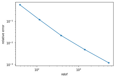
i =  0
err =  0.5595598334579617
i =  1
err =  0.11654484017074333
i =  2
err =  0.021448789398200045
i =  3
err =  0.0048565355595397075
i =  4
err =  0.001174815886669989

Convergence plot with matplotlib.

import matplotlib.pyplot as plt

plt.yscale('log')
plt.xscale('log')
plt.xlabel("ndof")
plt.ylabel("relative error")
ndof,err = zip(*l)
plt.plot(ndof,err, "-*")
plt.ion()
plt.show()

TDNNS method

Invert material law of Hooke and reset mesh.

def CMatInv(mat, E, nu):
    return (1+nu)/E*(mat-nu/(nu+1)*Trace(mat)*Id(2))

mesh = Mesh(sg.GenerateMesh(maxh=R/3))
mesh.Curve(order)
Draw(mesh)

BaseWebGuiScene

Instead of using Lagrangian elements together with an interpolation operator we can directly use H(curl) for the roation $\beta$.

order=1
if clamped:
    fesB = HCurl(mesh, order=order-1, dirichlet="circ", autoupdate=True)
    fesS = HDivDiv(mesh, order=order-1, dirichlet="", autoupdate=True)
else:
    fesB = HCurl(mesh, order=order-1)
    fesS = HDivDiv(mesh, order=order-1, dirichlet="circ", autoupdate=True)
fesW = H1(mesh, order=order, dirichlet="circ", autoupdate=True)

fes = FESpace( [fesW, fesB, fesS], autoupdate=True )
(u,beta,sigma), (du,dbeta,dsigma) = fes.TnT()

Use the TDNNS method with the stress (bending) tensor $\mathit{\sigma }$ as proposed in [Pechstein and Schöberl. The TDNNS method for Reissner-Mindlin plates. Numerische Mathematik 137, 3 (2017), 713-740] $$\begin{array}{rl}& \mathcal{L}(u,\beta ,\mathit{\sigma })=-\frac{6}{t^3}\Vert \mathit{\sigma }{\Vert }_{{\mathcal{C}}^{-1}}^2+⟨\mathit{\sigma },\mathrm{\nabla }\beta ⟩+\frac{tkG}{2}\Vert \mathrm{\nabla }u-\beta {\Vert }^2-{\int }_{\mathrm{\Omega }}f\cdot udx\\ & ⟨\mathit{\sigma },\mathrm{\nabla }\beta ⟩:=\sum _{T\in \mathcal{T}}{\int }_T\mathit{\sigma }:\mathrm{\nabla }\beta dx-{\int }_{\partial T}{\mathit{\sigma }}_{nn}{\beta }_{n}ds\end{array}$$

n = specialcf.normal(2)

a = BilinearForm(fes)
a += (-12/t**3*InnerProduct(CMatInv(sigma, E, nu),dsigma) + InnerProduct(dsigma,grad(beta)) + InnerProduct(sigma,grad(dbeta)))*dx
a += ( -((sigma*n)*n)*(dbeta*n) - ((dsigma*n)*n)*(beta*n) )*dx(element_boundary=True)
a += t*k*G*InnerProduct( grad(u)-beta, grad(du)-dbeta )*dx

f = LinearForm(fes)
f += -fz*du*dx

gfsol = GridFunction(fes, autoupdate=True)
gfu, gfbeta, gfsigma = gfsol.components

def SolveBVP():
    fes.Update()
    gfsol.Update()
    with TaskManager():
        a.Assemble()
        f.Assemble()
        inv = a.mat.Inverse(fes.FreeDofs())
        gfsol.vec.data = inv * f.vec

Solve, compute error, and refine.

l = []
for i in range(5):
    print("i = ", i)
    SolveBVP()
    if clamped:
        norm_w = sqrt(Integrate(w_c_ex*w_c_ex, mesh))
        err = sqrt(Integrate((gfu-w_c_ex)*(gfu-w_c_ex), mesh))/norm_w
    else:
        norm_w = sqrt(Integrate(w_s_ex*w_s_ex, mesh))
        err = sqrt(Integrate((gfu-w_s_ex)*(gfu-w_s_ex), mesh))/norm_w
    print("err = ", err)
    l.append ( (fes.ndof, err ))
    mesh.Refine()

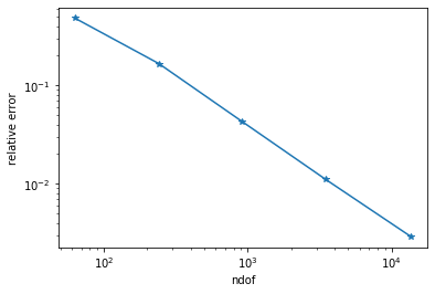
i =  0
err =  0.4806915268060298
i =  1
err =  0.1660840390786989
i =  2
err =  0.04302102327870844
i =  3
err =  0.011002228686409238
i =  4
err =  0.0028879335138407747

Convergence plot with matplotlib.

plt.yscale('log')
plt.xscale('log')
plt.xlabel("ndof")
plt.ylabel("relative error")
ndof,err = zip(*l)
plt.plot(ndof,err, "-*")

plt.ion()
plt.show()