This page was generated from unit-3.4-simplehyp/shallow2D.ipynb.

3.4 A Nonlinear conservation law: shallow water equation in 2D

We consider the shallow water equations as an example of a nonlinear conservation law, i.e. we consider

$$\partial_t \mathbf{U} + \operatorname{div}(\mathbf{F} (\mathbf{U} )) = 0 \qquad in \qquad \Omega \times[0,T],$$

with

$$\mathbf{U} = (h, \mathbf{w}) = (h, hu, hv) = (\mathbf{u}_1, \mathbf{u}_2, \mathbf{u}_3)$$

and

$$\begin{split}\mathbf{F}(\mathbf{U}) = \left( \begin{array}{c@{}c@{\qquad}c@{}c} h u & & h v & \\ h u^2 &+ \frac12 g h^2 & h u v & \\ h u v & & h v^2 & + \frac12 g h^2 \end{array} \right) = \left( \begin{array}{cc} \mathbf{u}_2 & \mathbf{u}_3 \\ \frac{\mathbf{u}_2^2}{\mathbf{u}_1} + \frac12 g \mathbf{u}_1^2 & \frac{\mathbf{u}_2 \mathbf{u}_3}{\mathbf{u}_1} \\ \frac{\mathbf{u}_2 \mathbf{u}_3}{\mathbf{u}_1} & \frac{\mathbf{u}_3^2}{\mathbf{u}_1} + \frac12 g \mathbf{u}_1^2 \end{array} \right) = \left( \begin{array}{cc} h \mathbf{w}^T \\ h \mathbf{w} \otimes \mathbf{w} + \frac12 g h^2 \mathbf{I} \end{array} \right)\end{split}$$

Jacobian of the flux for shallow water:

$$\begin{align*} \mathbf{A}_1 & = \left(\begin{array}{ccc} 0 & 1 & 0 \\ - \frac{\mathbf{u}_2^2}{\mathbf{u}_1^2} + g \mathbf{u}_1 & 2 \frac{\mathbf{u}_2}{\mathbf{u}_1} & 0 \\ - \frac{\mathbf{u}_2 \mathbf{u}_3}{\mathbf{u}_1^2} & \frac{\mathbf{u}_3}{\mathbf{u}_1} & \frac{\mathbf{u}_2}{\mathbf{u}_1} \end{array} \right) = \left( \begin{array}{ccc} 0 & 1 & 0 \\ - u^2 + g h & 2 u & 0 \\ - u v & v & u \end{array} \right) \end{align*}$$

$$\begin{align*} \mathbf{A}_2 & = \left( \begin{array}{ccc} 0 & 0 & 1 \\ - \frac{\mathbf{u}_2\mathbf{u}_3}{\mathbf{u}_1^2} & \frac{\mathbf{u}_3}{\mathbf{u}_1} & \frac{\mathbf{u}_2}{\mathbf{u}_1} \\ - \frac{\mathbf{u}_3^2}{\mathbf{u}_1^2} + g \mathbf{u}_1 & 0 & 2\frac{\mathbf{u}_3}{\mathbf{u}_1} \end{array} \right) = \left( \begin{array}{ccc} 0 & 0 & 1 \\ - uv & v & u \\ - v^2 + gh & 0 & 2 v \end{array} \right) \end{align*}$$

$$\begin{align*} \mathbf{A}(\mathbf{u}, \mathbf{n}) & = n_1 \mathbf{A}_1 + n_2 \mathbf{A}_2 = \left( \begin{array}{ccc} 0 & n_1 & n_2 \\ - u \alpha - g h n_1 & \alpha + u n_1 & u n_2 \\ - v \alpha - g h n_2 & v n_1 & \alpha + v n_2 \end{array} \right), \quad \text{ with } \alpha = (\mathbf{u}, \mathbf{n}), \end{align*}$$

spectrum:

$$\rho( \mathbf{A}(\mathbf{u}, \mathbf{n}) ) = \{ \alpha + \sqrt{g h}, \alpha, \alpha - \sqrt{g h} \}$$

from ngsolve import * # sloppy
from netgen import gui

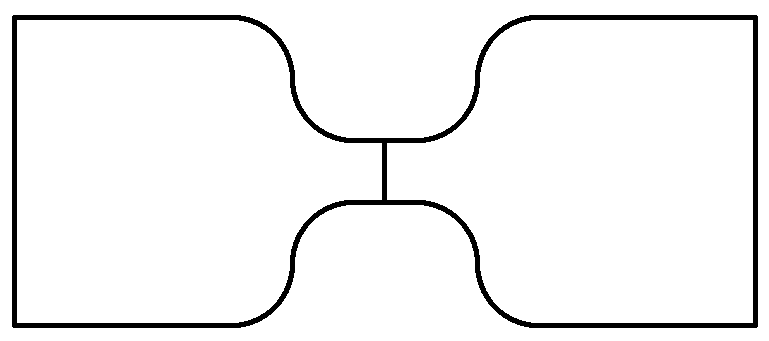
The dam break problem (geometry)

from netgen.geom2d import SplineGeometry
geo = SplineGeometry()

pnts =[ (-12,-5), (-7,-5), (-5,-5), (-3,-5), (-3,-3),
        (-3,-1), (-1,-1), ( 0,-1), ( 1,-1), ( 3,-1),
        ( 3,-3), ( 3,-5), ( 5,-5), ( 7,-5), ( 12,-5),
        ( 12, 5), ( 7, 5), ( 5, 5), ( 3, 5), ( 3, 3),
        ( 3, 1), ( 1, 1), ( 0, 1), (-1, 1), (-3, 1),
        (-3, 3), (-3, 5), (-5, 5), (-7, 5), (-12, 5)]
pnts = [geo.AppendPoint(*pnt) for pnt in pnts]

curves = [[["line",0,1],"wall",1, 0], [["line",1,2],"wall",1, 0],
          [["spline3",2,3,4],"wall",1, 0],[["spline3",4,5,6],"wall",1, 0],[["line",6,7],"wall",1, 0],
          [["line",7,22],"dam",1, 2],     # <--- dam interface
          [["line",7,8],"wall",2, 0],[["spline3",8,9,10],"wall",2, 0],
          [["spline3",10,11,12],"wall",2, 0],[["line",12,13],"wall",2, 0],[["line",13,14],"wall",2, 0],
          [["line",14,15],"wall",2, 0], # <--- right boundary
          [["line",15,16],"wall",2, 0],[["line",16,17],"wall",2, 0],
          [["spline3",17,18,19],"wall",2, 0],[["spline3",19,20,21],"wall",2, 0],
          [["line",21,22],"wall",2, 0],[["line",22,23],"wall",1, 0],
          [["spline3",23,24,25],"wall",1, 0],[["spline3",25,26,27],"wall",1, 0],
          [["line",27,28],"wall",1, 0],[["line",28,29],"wall",1, 0],
          [["line",29,0],"wall",1, 0]]   # <--- left boundary

for c,bc,l,r in curves:
    geo.Append(c,bc=bc,leftdomain=l, rightdomain=r)
geo.SetMaterial(1,"upperlevel")
geo.SetMaterial(2,"lowerlevel")

mesh = Mesh(geo.GenerateMesh(maxh=2))
mesh.Curve(3)
Draw(mesh)

Vectorial (dim=3) approximation space:

order = 2
fes = L2(mesh,order=order,dim=3)

initial and boundary conditions

U,V = fes.TnT() # "Trial" and "Test" function
h, hu, hv = U

# initial conditions
h0mat = {"upperlevel" : 10, "lowerlevel" : 2}
U0 = CoefficientFunction((CoefficientFunction([h0mat[mat] for mat in mesh.GetMaterials()]),0,0))

# boundary conditions
hbndreg = CoefficientFunction([{"wall" : h, "dam" : 0}[rg] for rg in mesh.GetBoundaries()])
hubndreg = CoefficientFunction([{"wall" : -hu, "dam" : 0}[rg] for rg in mesh.GetBoundaries()])
hvbndreg = CoefficientFunction([{"wall" : -hv, "dam" : 0}[rg] for rg in mesh.GetBoundaries()])

Ubnd = CoefficientFunction((hbndreg,hubndreg,hvbndreg))

# constant for gravitational force
g=1

Flux definition and numerical flux choice (Lax-Friedrich)

$$\begin{split}\mathbf{F}(\mathbf{U}) = \left( \begin{array}{c@{}c@{\qquad}c@{}c} h u & & h v & \\ h u^2 &+ \frac12 g h^2 & h u v & \\ h u v & & h v^2 & + \frac12 g h^2 \end{array} \right) = \left( \begin{array}{cc} \mathbf{u}_2 & \mathbf{u}_3 \\ \frac{\mathbf{u}_2^2}{\mathbf{u}_1} + \frac12 g \mathbf{u}_1^2 & \frac{\mathbf{u}_2 \mathbf{u}_3}{\mathbf{u}_1} \\ \frac{\mathbf{u}_2 \mathbf{u}_3}{\mathbf{u}_1} & \frac{\mathbf{u}_3^2}{\mathbf{u}_1} + \frac12 g \mathbf{u}_1^2 \end{array} \right) = \left( \begin{array}{cc} h \mathbf{w}^T \\ h \mathbf{w} \otimes \mathbf{w} + \frac12 g h^2 \mathbf{I} \end{array} \right)\end{split}$$

def F(U):
    h, hvx, hvy = U
    vx = hvx/h
    vy = hvy/h
    return CoefficientFunction(((hvx,hvy),
                                (hvx*vx + 0.5*g*h**2, hvx*vy),
                                (hvx*vy, hvy*vy + 0.5*g*h**2)),dims=(3,2))

$$\hat{\mathbf{F}}(\mathbf{U}) \cdot \mathbf{n} = \frac{(\mathbf{F}(\mathbf{U}^l)+\mathbf{F}(\mathbf{U}^r)}{2} \cdot \mathbf{n} + \frac{|\lambda|}{2} (\mathbf{U}^l - \mathbf{U}^r), \quad (\cdot^l: \text{current element}, \quad \cdot^r: \text{neighbor element})$$

n = specialcf.normal(mesh.dim)

def Max(u,v):
    return IfPos(u-v,u,v)
def Fmax(A,B): # max. characteristic speed:
    ha, hua, hva = A
    hb, hub, hvb = B
    vnorma = sqrt(hua**2+hva**2)/ha
    vnormb = sqrt(hub**2+hvb**2)/hb
    return Max(vnorma+sqrt(g*A[0]),vnormb+sqrt(g*B[0]))

def Fhatn(U): # numerical flux
    Uhat = U.Other(bnd=Ubnd)
    return (0.5*F(U)+0.5*F(Uhat))*n + Fmax(U,Uhat)/2*(U-Uhat)

DG formulation

We recall that a BilinearForm is allowed to be nonlinear in the first argument.

def DGBilinearForm(fes,F,Fhatn,Ubnd):
    a = BilinearForm(fes, nonassemble=True)
    a += - InnerProduct(F(U),Grad(V)) * dx
    a += InnerProduct(Fhatn(U),V) * dx(element_boundary=True)
    return a

a = DGBilinearForm(fes,F,Fhatn,Ubnd)

Simple fix to deal with shocks: artificial diffusion:

from DGdiffusion import AddArtificialDiffusion

artvisc = Parameter(1.0)
if order > 0:
    AddArtificialDiffusion(a,Ubnd,artvisc,compile=True)

Visualization of solution quantities

gfu = GridFunction(fes)
gfh, gfhu, gfhv = gfu
gfvu = gfhu/gfh
gfvv = gfhv/gfh
momentum = CoefficientFunction((gfhu,gfhv))
velocity = CoefficientFunction((gfvu,gfvv))
gfu.Set(U0)
Draw(momentum,mesh,"mom")
Draw(velocity,mesh,"vel")
Draw(gfh,mesh,"h")

Explicit Euler time stepping

def TimeLoop(a,gfu,dt,T,nsamplings=100):
    #gfu.Set(U0)
    res = gfu.vec.CreateVector()
    fes = a.space
    t = 0; i = 0
    nsteps = int(ceil(T/dt))
    invma = fes.Mass(1).Inverse() @ a.mat
    with TaskManager():
        while t <= T - 0.5*dt:
            res = invma * gfu.vec
            gfu.vec.data -= dt * res
            t += dt
            if (i+1) % int(nsteps/nsamplings) == 0:
                Redraw()
            i+=1
            print("\rt = {:.10}".format(t),end="")
    Redraw()

TimeLoop(a,gfu,dt=0.0004,T=3)

t = 3.0

You may play around with this example.

• change the artificial diffusion parameter: How does it influence the solution

• change boundary conditions: left boundary -> fixed height and non-reflecting

• change the initial heights

• introduce a (circular) obstacle below the dam

• Generate output to create a video: To this end take a look at the final unit of this section.

%%HTML
<video width="600" height="400" controls>
    <source src="../../_static/shallow2D.mov">
</video>