This page was generated from unit-1.6-adaptivity/adaptivity.ipynb.
1.6 Error estimation & adaptive refinement
In this tutorial, we apply a Zienkiewicz-Zhu type error estimator and run an adaptive loop with these steps:
[1]:
import netgen.gui
from ngsolve import *
from netgen.geom2d import SplineGeometry
import matplotlib.pyplot as plt
Geometry
The following geometry represents a heated chip embedded in another material that conducts away the heat.
[2]:
#   point numbers 0, 1, ... 11
#   sub-domain numbers (1), (2), (3)
#
#
#             7-------------6
#             |             |
#             |     (2)     |
#             |             |
#      3------4-------------5------2
#      |                           |
#      |             11            |
#      |           /   \           |
#      |         10 (3) 9          |
#      |           \   /     (1)   |
#      |             8             |
#      |                           |
#      0---------------------------1
#

def MakeGeometry():
    geometry = SplineGeometry()

    # point coordinates ...
    pnts = [ (0,0), (1,0), (1,0.6), (0,0.6), \
             (0.2,0.6), (0.8,0.6), (0.8,0.8), (0.2,0.8), \
             (0.5,0.15), (0.65,0.3), (0.5,0.45), (0.35,0.3) ]
    pnums = [geometry.AppendPoint(*p) for p in pnts]

    # start-point, end-point, boundary-condition, left-domain, right-domain:
    lines = [ (0,1,1,1,0), (1,2,2,1,0), (2,5,2,1,0), (5,4,2,1,2), (4,3,2,1,0), (3,0,2,1,0), \
              (5,6,2,2,0), (6,7,2,2,0), (7,4,2,2,0), \
              (8,9,2,3,1), (9,10,2,3,1), (10,11,2,3,1), (11,8,2,3,1) ]

    for p1,p2,bc,left,right in lines:
        geometry.Append(["line", pnums[p1], pnums[p2]], bc=bc, leftdomain=left, rightdomain=right)

    geometry.SetMaterial(1,"base")
    geometry.SetMaterial(2,"chip")
    geometry.SetMaterial(3,"top")

    return geometry

mesh = Mesh(MakeGeometry().GenerateMesh(maxh=0.2))
Spaces & forms
The problem is to find \(u\) in \(H_{0,D}^1\) satisfying
for all \(v\) in \(H_{0,D}^1\). We expect the solution to have singularities due to the nonconvex re-enrant angles and discontinuities in \(\lambda\).
[3]:
fes = H1(mesh, order=3, dirichlet=[1])
u, v = fes.TnT()

# one heat conductivity coefficient per sub-domain
lam = CoefficientFunction([1, 1000, 10])
a = BilinearForm(fes)
a += lam*grad(u)*grad(v)*dx

# heat-source in inner subdomain
f = LinearForm(fes)
f += CoefficientFunction([0, 0, 1])*v * dx

c = Preconditioner(a, type="multigrid", inverse="sparsecholesky")

gfu = GridFunction(fes)
Draw (gfu)
Note that the linear system is not yet assembled above.
Solve
Since we must solve multiple times, we define a function to solve the boundary value problem, where assembly, update, and solve occurs.
[4]:
def SolveBVP():
    fes.Update()
    gfu.Update()
    a.Assemble()
    f.Assemble()
    inv = CGSolver(a.mat, c.mat)
    gfu.vec.data = inv * f.vec
    Redraw (blocking=True)
[5]:
SolveBVP()
Estimate
We implement a gradient-recovery-type error estimator. For this, we need an H(div) space for flux recovery. We must compute the flux of the computed solution and interpolate it into this H(div) space.
[6]:
space_flux = HDiv(mesh, order=2)
gf_flux = GridFunction(space_flux, "flux")

flux = lam * grad(gfu)
gf_flux.Set(flux)
Element-wise error estimator: On each element \(T\), set
where \(u_h\) is the computed solution gfu and \(I_h\) is the interpolation performed by Set in NGSolve.
[7]:
err = 1/lam*(flux-gf_flux)*(flux-gf_flux)
Draw(err, mesh, 'error_representation')
[8]:
eta2 = Integrate(err, mesh, VOL, element_wise=True)
print(eta2)
 1.40235e-10
 2.49521e-08
 4.66339e-06
 3.44351e-10
 6.11669e-10
 1.70842e-08
 2.49781e-08
 1.74657e-07
 1.16017e-07
 2.56058e-07
 2.16996e-07
 7.85551e-10
 6.09821e-07
 4.07856e-06
 5.50921e-07
 3.39019e-08
 9.47374e-07
 3.22632e-06
 1.78077e-07
 7.08956e-07
 3.54306e-08
 1.40757e-06
 1.65881e-08
 6.80644e-07
 3.71548e-08
 2.54721e-07
 4.46692e-09
 1.61318e-06
 4.8288e-10
 6.82924e-07
 7.9077e-10
 4.24959e-07
 1.11462e-10
 1.04737e-11
 3.71384e-10
 1.43675e-11
 2.37229e-10
 4.96356e-12
 8.54661e-07
 8.18303e-07
The above values, one per element, lead us to identify elements which might have large error.
Mark
We mark elements with large error estimator for refinement.
[9]:
maxerr = max(eta2)
print ("maxerr = ", maxerr)

for el in mesh.Elements():
    mesh.SetRefinementFlag(el, eta2[el.nr] > 0.25*maxerr)

Draw(gfu)
maxerr = 4.663388089339081e-06
Automate the above steps
[11]:
l = []    # l = list of estimated total error

def CalcError():

    # compute the flux:
    space_flux.Update()
    gf_flux.Update()
    flux = lam * grad(gfu)
    gf_flux.Set(flux)

    # compute estimator:
    err = 1/lam*(flux-gf_flux)*(flux-gf_flux)
    eta2 = Integrate(err, mesh, VOL, element_wise=True)
    maxerr = max(eta2)
    l.append ((fes.ndof, sqrt(sum(eta2))))
    print("ndof =", fes.ndof, " maxerr =", maxerr)

    # mark for refinement:
    for el in mesh.Elements():
        mesh.SetRefinementFlag(el, eta2[el.nr] > 0.25*maxerr)
[12]:
CalcError()
mesh.Refine()
ndof = 433 maxerr = 2.6978168422478246e-06
Run the adaptive loop
[13]:
while fes.ndof < 50000:
    SolveBVP()
    CalcError()
    mesh.Refine()
ndof = 526  maxerr = 9.202560088708061e-07
ndof = 1108  maxerr = 3.330204916900337e-07
ndof = 1891  maxerr = 1.2062317553466168e-07
ndof = 2680  maxerr = 4.37214705841322e-08
ndof = 3538  maxerr = 2.0339203720066086e-08
ndof = 4309  maxerr = 1.0151987890612577e-08
ndof = 4819  maxerr = 5.071194420271339e-09
ndof = 5428  maxerr = 2.533785850989227e-09
ndof = 6118  maxerr = 1.2661665048716232e-09
ndof = 6547  maxerr = 6.327658735072703e-10
ndof = 7291  maxerr = 3.1623214954898227e-10
ndof = 8059  maxerr = 1.5804152813931348e-10
ndof = 8779  maxerr = 7.898486052529126e-11
ndof = 9718  maxerr = 3.947505265907015e-11
ndof = 11263  maxerr = 1.9728271994609e-11
ndof = 12259  maxerr = 9.859752755765394e-12
ndof = 13726  maxerr = 4.927669994099061e-12
ndof = 15889  maxerr = 2.4627571067698184e-12
ndof = 18301  maxerr = 1.23083840141265e-12
ndof = 20839  maxerr = 6.151360541146951e-13
ndof = 23818  maxerr = 3.074324043686468e-13
ndof = 28522  maxerr = 1.5364845126901105e-13
ndof = 32227  maxerr = 7.678665530988363e-14
ndof = 38272  maxerr = 3.837655732658751e-14
ndof = 44662  maxerr = 1.9179195909549555e-14
ndof = 51457  maxerr = 9.585184358669049e-15
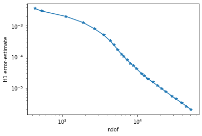
Plot history of adaptive convergence
[14]:
plt.yscale('log')
plt.xscale('log')
plt.xlabel("ndof")
plt.ylabel("H1 error-estimate")
ndof,err = zip(*l)
plt.plot(ndof,err, "-*")

plt.ion()
plt.show()