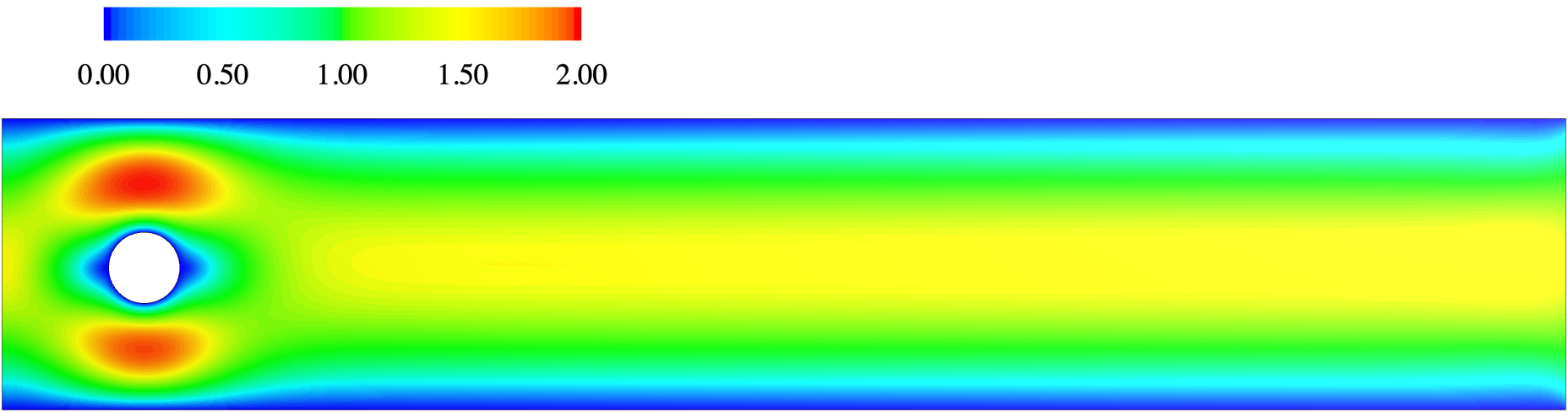
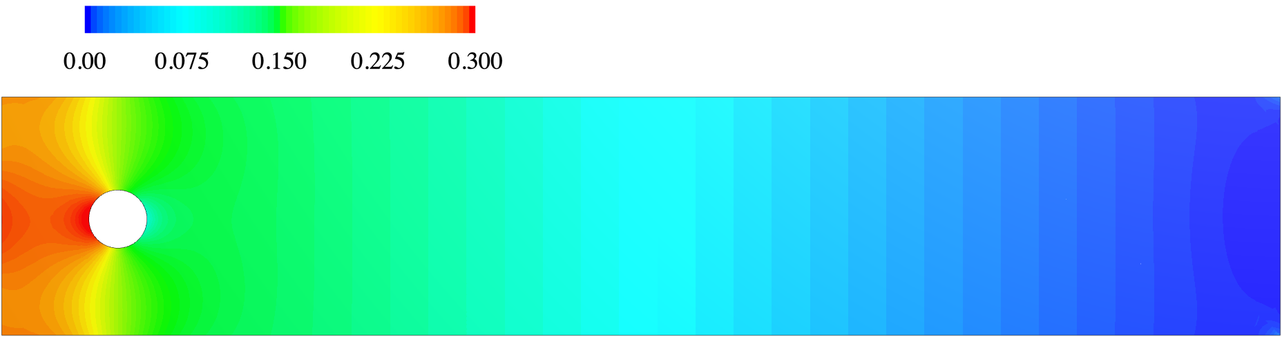
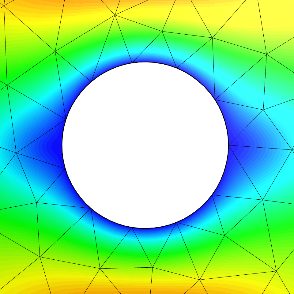
ngsolve.webgui at visualization order 4 on the curved mesh
(mesh.Curve(3)). Right: zoom on the cylinder with the
curved elements. The pressure difference between the front and back of
the cylinder is \(p(0.15,0.2)-p(0.25,0.2) =
0.229\).NGSolve Technical Note 2026-03 \(\bullet\) November 2026
We consider the Stokes problem with viscosity \(\nu\): \[-\operatorname{div}\bigl(2\nu\,\varepsilon(u)\bigr) + \nabla p = f, \qquad \operatorname{div} u = 0 \quad\text{in } \Omega,\] with Dirichlet data \(u = g\) on \(\Gamma_D\) and the do-nothing condition \((2\nu\varepsilon(u) - pI)\,n = 0\) on \(\Gamma_N\). The MCS method [2, 1] introduces the deviatoric viscous stress \(\sigma = 2\nu \operatorname{dev}\varepsilon(u)\) as an additional unknown. Its main properties are:
The velocity is \(H(\operatorname{div})\)-conforming and the pressure space is exactly \(\operatorname{div} V_h\), so \(\operatorname{div} u_h = 0\) pointwise. The method is pressure robust: velocity errors do not depend on \(p/\nu\).
The stress is normal-tangential continuous (\(\sigma \in H(\operatorname{curl}\operatorname{div})\)). Through \(\sigma_{nt}\), it enforces the missing tangential continuity of \(u_h\) weakly.
Hybridization by a facet variable \(\hat u\) (the tangential velocity) makes all stress and higher-order velocity/pressure dofs element-local. After static condensation only facet unknowns remain.
Symmetry of \(\sigma\) is imposed weakly by a skew-symmetric Lagrange multiplier \(\eta\) (MCS with weak symmetry [3]). Without it, one uses the simpler gradient form \(\sigma = \nu\operatorname{dev}\nabla u\).
Find \((u_h,\sigma_h,\hat u_h,p_h,\eta_h) \in V_h\times\Sigma_h^{dc}\times\hat V_h\times Q_h\times W_h\) such that for all test functions \[\begin{aligned} \tfrac{1}{2\nu}(\sigma_h,\tau) - b(\tau,(u_h,\hat u_h)) + (\tau,\eta_h) &= 0 && \forall\, \tau \in \Sigma_h^{dc},\\ -b(\sigma_h,(v,\hat v)) + (\operatorname{div} v, p_h) &= -(f,v) && \forall\, (v,\hat v) \in V_h\times\hat V_h,\\ (\operatorname{div} u_h, q) = 0, \qquad (\sigma_h,\xi) &= 0 && \forall\, q\in Q_h,\ \xi\in W_h, \end{aligned}\] with the distributional divergence pairing, written element by element: \[b(\tau,(v,\hat v)) \;=\; \sum_{T\in\mathcal{T}_h}\Bigl( \int_T \tau : \nabla v \,dx \;-\; \int_{\partial T} (\tau n)_t\cdot(v_t - \hat v_t)\,ds \Bigr), \qquad w_t := w - (w\cdot n)\,n .\] The first equation states \(\sigma_h = 2\nu(\operatorname{dev}\nabla u_h - \eta_h)\). Together with \((\sigma_h,\xi)=0\) this gives \(\eta_h \approx \operatorname{skw}\nabla u_h\), hence \(\sigma_h \approx 2\nu\operatorname{dev}\varepsilon(u_h)\). For the gradient form, drop \(\eta,\xi\) and replace \(\tfrac{1}{2\nu}\) by \(\tfrac1\nu\). The velocity Dirichlet condition is split: \(u\cdot n = g\cdot n\) on \(V_h\) and \(\hat u = g_t\) on \(\hat V_h\). The do-nothing condition is natural.
Let \(k\ge 1\) be the velocity order, \(\mathcal{T}_h\) the mesh and \(\mathcal{F}_h\) its facets. All spaces below are created from the velocity space alone. The order rules have been checked to be stable (injectivity of the discrete divergence, optimal convergence) on trigs, quads, tets, prisms and hexes.
V = HDiv(mesh, order=k). On simplices the default is
BDM: \(V_h = \{v\in H(\operatorname{div}):
v|_T \in P_k(T)^d\}\). On quads, prisms and hexes the default is
the tensor-product Raviart–Thomas element. For prisms this is \(RT_k(\text{trig})\otimes P_k \,\oplus\,
P_k(\text{trig})\otimes P_{k+1}\,e_z\). The flag
RT=True/False (or trigRT, tetRT,
… per element type) overrides the default; see Technical Note
2026-01.
Q = V.CreateDivergenceSpace() gives \(Q_h = \operatorname{div} V_h\) exactly,
element by element: \(P_{k-1}(T)\) for
BDM, and for RT \(P_k(T)\) on
simplices, \(Q_k\) on quads/hexes,
\(P_k\otimes P_k\) on prisms. Element
constants are global (wirebasket) dofs. All higher modes are local, so
they are removed by static condensation.
S = V.CreateStressSpace() returns
HCurlDiv(mesh, order=k-1, orderinner=k): \[\Sigma_h=\Bigl\{\tau\in L^2(\Omega)^{d\times d}:\
\begin{aligned}[t]&\operatorname{tr}\tau=0,\ \ \tau|_T \text{
polynomial of degree }k,\\
&\tau_{nt}:=(\tau n)_t \text{ continuous across }
\mathcal{F}_h,\ \ \tau_{nt}|_F\in
P_{k-1}(F)^{d-1}\Bigr\},\end{aligned}\] with \(Q_{k-1}(F)\) on quadrilateral facets. On
simplices, \(\Sigma_h =
\{\tau\in\operatorname{dev}P_k:\ \tau_{nt}|_F\in P_{k-1}\}\) is
the original MCS stress space. The same space serves the gradient form
and the weakly symmetric form. A computed inf-sup constant of the full
system shows no need for the Gopalakrishnan–Guzmán bubbles [4] there, on trigs and tets alike. The only special
case is RT velocities of order \(1\) on
trigs. There orderinner=1 plus GGbubbles is
used: 8 local dofs instead of 12 for orderinner=2, with the
same quadrature order. To inspect what was chosen, use
print(S.flags). An explicit order=... switches
the automatic choice off. Other keyword arguments are passed to
HCurlDiv.
Sdc = Discontinuous(S) breaks the \(\tau_{nt}\)-continuity, so \(\Sigma_h^{dc} = \prod_T \Sigma_h|_T\)
consists of local dofs only. Sdc.base_space gives back the
conforming space S.
Vhat = Sdc.CreateMultiplierSpace() is
TangentialFacetFESpace(mesh, order=k-1): \[\hat V_h = \{\hat v \in L^2(\mathcal{F}_h)^d:\
\hat v\cdot n = 0,\ \ \hat v|_F \in P_{k-1}(F)^{d-1}\}.\] Its
degree matches \(\tau_{nt}\) exactly.
Therefore \(\{\tau \in \Sigma_h^{dc}:
\sum_T\int_{\partial T}\tau_{nt}\cdot\hat v = 0\ \forall \hat v\} =
\Sigma_h\), and the hybrid and the conforming method give
identical solutions.
W = Sdc.base_space.CreateSymmetryMultiplierSpace() is
MatrixValued(L2(mesh, order=k-1), skewsymmetric=True):
\[W_h = \{\eta \in L^2(\Omega)^{d\times d}:\
\eta = -\eta^T,\ \eta|_T\in P_{k-1}(T)\}.\] Its proxy is a
skew-symmetric matrix, so the constraint is just
InnerProduct(sigma, xi)*dx.
| element | velocity default | \(Q_h\) | \(\Sigma_h\) (facet, inner) |
|---|---|---|---|
| trig | BDM\(_k\) | \(P_{k-1}\) | \((k-1,\,k)\); RT\(_1\): \((0,1)\) + GG bubbles |
| quad | RT\(_k\) (tensor) | \(Q_k\) | \((k-1,\,k)\) |
| tet | BDM\(_k\) | \(P_{k-1}\) | \((k-1,\,k)\) |
| prism | RT\(_k\) (tensor) | \(P_k\otimes P_k\) | \((k-1,\,k)\) |
| hex | RT\(_k\) (tensor) | \(Q_k\) | \((k-1,\,k)\) |
Stokes flow around a cylinder in the DFG channel. The velocity order
is \(k=3\), with weak symmetry and
hybridization. Solve detects the local dofs and applies
static condensation automatically.
from ngsolve import *
from netgen.occ import Rectangle, Circle, X, Y

rect = Rectangle(2.2, 0.41).Face()
rect.edges.Min(X).name = "inlet"
rect.edges.Max(X).name = "outlet"
rect.edges.Min(Y).name = rect.edges.Max(Y).name = "wall"
cyl = Circle((0.2, 0.2), 0.05).Face()
cyl.edges.name = "cyl"
mesh = (rect - cyl).GenerateMesh(dim=2, maxh=0.05)
mesh.Curve(3)

k, nu = 3, 1e-3
V    = HDiv(mesh, order=k)                                 # velocity
S    = Discontinuous(V.CreateStressSpace())                # stress, hybridized
Vhat = S.CreateMultiplierSpace()                           # tangential velocity
Q    = V.CreateDivergenceSpace()                           # pressure = div V
W    = S.base_space.CreateSymmetryMultiplierSpace()        # skew-symmetric multiplier

(u, sigma, uhat, p, eta), (v, tau, vhat, q, xi) = (V*S*Vhat*Q*W).TnT()

n = specialcf.normal(2)
tang = lambda w: w - (w*n)*n
def B(tau, v, vhat):
    return InnerProduct(tau, Grad(v))*dx - tang(tau*n)*tang(v-vhat)*dx(element_boundary=True)

a = (1/(2*nu)*InnerProduct(sigma, tau)*dx - B(tau, u, uhat) - B(sigma, v, vhat)
     + div(u)*q*dx + div(v)*p*dx
     + InnerProduct(sigma, xi)*dx + InnerProduct(tau, eta)*dx)

uin = CF((1.5*4*y*(0.41-y)/0.41**2, 0))
gf = Solve(a == 0, u[BND("inlet")] == uin, uhat[BND("inlet")] == uin,
           u[BND("wall|cyl")] == 0, uhat[BND("wall|cyl")] == 0)
uh, sh, ph = gf[u], gf[sigma], gf[p]
For a body force, write a == -f*v*dx. Without weak
symmetry, drop W, eta, xi and use
1/nu in the first term. The space V*S*Vhat*Q*W
has 47 840 dofs; after condensation only the facet dofs of
V and Vhat and the element constants of
Q remain. The run takes about one second on a laptop. The
computed velocity satisfies \(\|\operatorname{div}u_h\|_{L^2} =
6\cdot10^{-15}\).
ngsolve.webgui at visualization order 4 on the curved mesh
(mesh.Curve(3)). Right: zoom on the cylinder with the
curved elements. The pressure difference between the front and back of
the cylinder is \(p(0.15,0.2)-p(0.25,0.2) =
0.229\).Manufactured solution \(u = \operatorname{curl}\psi\) with \(\psi = (x(1-x)y(1-y))^2\) on the unit square, and the analogous field on the unit cube. The pressure is \(p = x - \tfrac12\). Weakly symmetric form, errors \(\|u-u_h\|_{L^2}\) and \(\|\operatorname{dev}(2\varepsilon(u)) - \sigma_h\|_{L^2}\), rates in brackets.
| mesh | \(k\) | \(h=1/4\) | \(1/8\) | \(1/16\) | \(1/32\) |
|---|---|---|---|---|---|
| trig (BDM) | 1 | 1.04e-3 / 2.82e-2 | 2.49e-4 (2.1) / 1.47e-2 (0.9) | 5.31e-5 (2.2) / 7.07e-3 (1.1) | 1.35e-5 (2.0) / 3.55e-3 (1.0) |
| 2 | 2.34e-4 / 7.92e-3 | 2.28e-5 (3.4) / 1.68e-3 (2.2) | 2.07e-6 (3.5) / 3.51e-4 (2.3) | 2.51e-7 (3.0) / 8.56e-5 (2.0) | |
| 3 | 2.14e-5 / 8.48e-4 | 1.14e-6 (4.2) / 9.28e-5 (3.2) | 6.00e-8 (4.2) / 1.12e-5 (3.1) | 3.20e-9 (4.2) / 1.18e-6 (3.2) | |
| mesh | \(k\) | \(h=1/2\) | \(1/4\) | \(1/8\) | |
| prism (RT) | 1 | 1.72e-4 / 3.06e-3 | 8.48e-5 (1.0) / 2.17e-3 (0.5) | 2.10e-5 (2.0) / 1.15e-3 (0.9) | |
| 2 | 9.26e-5 / 1.87e-3 | 1.22e-5 (2.9) / 5.92e-4 (1.7) | 1.64e-6 (2.9) / 1.59e-4 (1.9) |
The code is dimension independent. A duct with two prism boundary
layers on the walls and tets inside needs a different geometry and
specialcf.normal(3); the rest stays the same:
from netgen.occ import Box, X
from netgen.meshing import BoundaryLayerParameters

box = Box((0,0,0), (2,0.5,0.5))
box.faces.Min(X).name = "inlet"
box.faces.Max(X).name = "outlet"
box.faces[2:].name = "wall"
bl = BoundaryLayerParameters(boundary="wall", thickness=[0.02, 0.03])
mesh = box.GenerateMesh(maxh=0.15, boundary_layers=[bl])
# ... spaces and forms as above, n = specialcf.normal(3), k = 2
uin = CF((16*y*(0.5-y)*z*(0.5-z)/0.5**4, 0, 0))
gf = Solve(a == 0, u[BND("inlet|wall")] == uin, uhat[BND("inlet|wall")] == uin)
The mesh has 672 prisms and 506 tets, giving 239 436 dofs; the solve takes 11 s. The results are \(\|\operatorname{div}u_h\|_{L^2} = 1\cdot10^{-14}\) and a net flux below \(10^{-17}\) through the duct. The centreline velocity \(0.93\) is that of the developed duct profile.
Boundary conditions.
u[BND(..)] == g sets the normal component,
uhat[BND(..)] == g the tangential one. Both are needed for
no-slip and inflow. Leaving a boundary out of both gives the do-nothing
outflow.
Pure Dirichlet problems. The pressure is
determined only up to a constant. Fix it, e.g. by a
NumberSpace multiplier for \(\int
p = 0\) or a tiny \(-\varepsilon\,(p,q)\) term.
Exact mass conservation. \(\operatorname{div} u_h = 0\) holds
pointwise because Q is exactly \(\operatorname{div}\)V. Mixing
an RT velocity with a pressure of order \(k-1\) loses this property; always use
CreateDivergenceSpace().
Equivalence to the conforming method. The hybrid
and the conforming formulation (S instead of
Discontinuous(S), no Vhat) give the same \(u_h\). On conforming stresses, \(\hat u\) drops out of \(b\).
Interpolation.
gf.Set(cf, dual=True) uses the HCurlDiv dual basis (facet
moments of \(\tau_{nt}\) and interior
moments). It reproduces discrete fields exactly, also on prisms and on
curved or non-affine elements.
Element support. CreateStressSpace
handles trigs, quads, tets, prisms and hexes, also on mixed meshes;
pyramids raise an exception. The HCurlDiv prism is based on the element
by X. Mooslechner. Tet–prism interfaces are \(\tau_{nt}\)-conforming. Boundary values for
\(\hat u\) on quadrilateral faces
(hexes, prism layers) are supported.
P. L. Lederer. A Mass Conserving Mixed Stress Formulation for Incompressible Flows. PhD thesis, TU Wien, 2019.
J. Gopalakrishnan, P. L. Lederer and J. Schöberl. A mass conserving mixed stress formulation for the Stokes equations. IMA J. Numer. Anal. 40(3):1838–1874, 2020.
J. Gopalakrishnan, P. L. Lederer and J. Schöberl. A mass conserving mixed stress formulation for Stokes flow with weakly imposed stress symmetry. SIAM J. Numer. Anal. 58(1):706–732, 2020.
J. Gopalakrishnan and J. Guzmán. A second elasticity element using the matrix bubble. IMA J. Numer. Anal. 32(1):352–372, 2012.