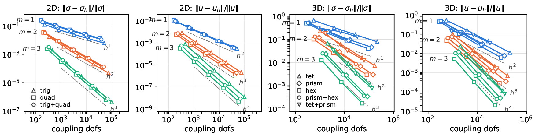
HCurl(m) with
CreateStressSpace(): relative \(L^2\) errors over the number of coupling
dofs. Dashed: optimal rates \(h^m\) for
\(\sigma\) and \(h^{m+1}\) for \(u\).NGSolve Technical Note 2026-02 \(\bullet\) November 2026
We consider linear elasticity on \(\Omega\subset\mathbb R^d\), \(d=2,3\): find the displacement \(u\) and the symmetric stress \(\sigma\) with \[A\sigma = \varepsilon(u), \qquad -\operatorname{div}\sigma = f \quad\text{in }\Omega, \qquad A\sigma := \tfrac{1}{2\mu}\bigl(\sigma - \tfrac{\lambda}{2\mu+d\lambda}\operatorname{tr}(\sigma)\,I\bigr),\] \(u=g\) on \(\Gamma_D\) and \(\sigma n = t\) on \(\Gamma_N\). Here \(\varepsilon(u)\) is the symmetric gradient and \(\mu,\lambda\) are the Lamé parameters. The tangential-displacement normal-normal-stress (TDNNS) method [1, 2] uses
a tangentially continuous displacement, \(u_h\in V_h\subset H(\operatorname{curl})\) (Nédélec elements), and
a symmetric stress with continuous normal-normal component \(\sigma_{nn}=n^T\sigma n\), \(\sigma_h\in\Sigma_h\subset H(\operatorname{div}\operatorname{div})\).
With \(w_t := w-(w\cdot n)n\), \(w_n:=w\cdot n\) and \(\tau_{nt}:=(\tau n)_t\), the method reads: find \((\sigma_h,u_h)\in\Sigma_h\times V_h\) such that \[\begin{aligned} (A\sigma_h,\tau) + \langle\operatorname{div}\tau,u_h\rangle &= \textstyle\int_{\Gamma_D} g_n\,\tau_{nn}\,ds && \forall\,\tau\in\Sigma_h,\\ \langle\operatorname{div}\sigma_h,v\rangle &= -(f,v) - \textstyle\int_{\Gamma_N} t_t\cdot v_t\,ds && \forall\,v\in V_h, \end{aligned}\] with the distributional divergence pairing, written element by element in two equivalent ways: \[\langle\operatorname{div}\tau,v\rangle \;=\; \sum_{T\in\mathcal{T}_h}\Bigl(\int_T \operatorname{div}\tau\cdot v\,dx - \int_{\partial T}\tau_{nt}\cdot v_t\,ds\Bigr) \;=\; -\sum_{T\in\mathcal{T}_h}\Bigl(\int_T \tau:\varepsilon(v)\,dx - \int_{\partial T}\tau_{nn}\,v_n\,ds\Bigr).\] The conditions \(u_t=g_t\) and \(\sigma_{nn}=t_n\) are essential; \(u_n = g_n\) and \(\sigma_{nt}=t_t\) are natural. The method is stable in \(h\)-dependent and in natural norms [2, 4] and it is suited for anisotropic elements in thin structures [3].
The \(nn\)-continuity of the stress is broken, \(\Sigma_h^{dc}=\prod_T\Sigma_h|_T\), and enforced by a multiplier \(\hat u_h\in\hat V_h\) on the facets \(\mathcal{F}_h\), which is the normal displacement. The pairing becomes \[\langle\operatorname{div}\tau,(v,\hat v)\rangle \;=\; \sum_{T\in\mathcal{T}_h}\Bigl(\int_T \operatorname{div}\tau\cdot v\,dx - \int_{\partial T}\tau_{nt}\cdot v_t\,ds - \int_{\partial T}\tau_{nn}\,\hat v_n\,ds\Bigr).\] Now both displacement conditions are essential (\(u_t=g_t\) in \(V_h\), \(\hat u_n=g_n\) in \(\hat V_h\)) and the whole traction is natural: the right-hand side gets \(-\int_{\Gamma_N}(t_t\cdot v_t+t_n\hat v_n)\,ds\). Prescribing only \(\hat u_n=0\) gives a sliding condition. All stress dofs are element-local; static condensation leaves a symmetric positive definite system for \((u_h,\hat u_h)\), after multiplying the equations by \(-1\) as in the listing below.
Let \(m\ge1\) be the displacement
order. The order conventions of HCurl are those of
Technical Note 2026-01 (High-order de Rham sequences on mixed
meshes): HCurl(m) has tangential traces of degree
\(m\) and contains the gradients of
H1(m+1); type1=True uses the gradients of
H1(m) only.
Q = HCurl(mesh, order=m) (default, Nédélec type II on
simplices) or HCurl(mesh, order=m, type1=True).
S = Q.CreateStressSpace() returns an
HDivDiv space of symmetric matrices with continuous \(\sigma_{nn}\), mapped by the double Piola
transformation. The polynomial degree of \(\sigma_{nn}\) on facets and the degree in
the element interior are chosen per element type (Table 1). print(S.flags) shows the
choice. Keyword arguments are passed to HDivDiv;
dirichlet="..." marks the boundary where \(\sigma_{nn}\) is essential (conforming
method), and an explicit order=... switches the automatic
choice off.
Sdc = Discontinuous(S) breaks the \(nn\)-continuity.
M = Sdc.CreateMultiplierSpace() is
NormalFacetFESpace with the facet order of S:
\(\hat V_h=\{\hat v\,n:\ \hat v|_F\in
P_k(F)\}\) (\(Q_k\) on
quadrilateral faces). Since the degrees match, the hybrid and the
conforming method give the same solution; measured differences are \(10^{-13}\) on tets, prisms, tet–prism,
prism–hex and trig–quad meshes.
| element | type1=True |
default HCurl(m)(single type
/ in mixed meshes) |
\(\sigma\) dofs | \(u\) dofs |
|---|---|---|---|---|
| trig | \((m{-}1,\,m{-}1)\), plus |
\((m,\,m)\) / \((m{-}1,\,m)\) | 18 | 12 |
| quad | \((m{-}1,\,m{-}1)\) | \((m{-}1,\,m{-}1)\),
quadfullpol |
25 | 19 |
| tet | \((m{-}1,\,m{-}1)\) | \((m{-}1,\,m{-}1)\), plus |
36 | 30 |
| prism | \((m{-}1,\,m{-}1)\) | \((m,\,m)\) / \((m{-}1,\,m)\) | 131 | 58 |
| hex | \((m{-}1,\,m{-}1)\) | \((m{-}1,\,m)\) | 228 | 91 |
Hybrid TDNNS on unstructured tets, \(m=2\), manufactured solution: displacement
data on five faces of the unit cube, traction data on the sixth.
Solve detects the local dofs and applies static
condensation.
from ngsolve import *
from netgen.occ import Box, X
box = Box((0,0,0), (1,1,1))
box.faces.name = "fix"
box.faces.Max(X).name = "load"
mesh = box.GenerateMesh(maxh=0.2)

k, E, nu = 2, 1, 0.3
mu, lam = E/(2*(1+nu)), E*nu/((1+nu)*(1-2*nu))
A = lambda s: 1/(2*mu)*(s - lam/(2*mu+3*lam)*Trace(s)*Id(3))    # compliance

uex = CF((sin(x+y)*(1+z), cos(x)*y+z*z, exp(x)*sin(z)+y))       # manufactured solution
gradu = CF((uex.Diff(x), uex.Diff(y), uex.Diff(z)), dims=(3,3)).trans
sex = 2*mu*Sym(gradu) + lam*Trace(gradu)*Id(3)
f = -CF(tuple(sex[i,0].Diff(x) + sex[i,1].Diff(y) + sex[i,2].Diff(z) for i in range(3)))

Q = HCurl(mesh, order=k)                    # displacement, tangentially continuous
S = Discontinuous(Q.CreateStressSpace())    # stress, nn-continuity broken
M = S.CreateMultiplierSpace()               # normal displacement on facets
(sigma, u, un), (tau, v, vn) = (S*Q*M).TnT()
n = specialcf.normal(3)
tang = lambda w: w - (w*n)*n
nn = lambda s: (s*n)*n
def b(tau, v, vn):                          # -<div tau, (v, vn)>
    return -div(tau)*v*dx + ((tau*n)*tang(v) + nn(tau)*(vn*n))*dx(element_boundary=True)
a = -InnerProduct(A(sigma), tau)*dx + b(tau, u, un) + b(sigma, v, vn)
rhs = f*v*dx + (sex*n)*(tang(v.Trace()) + vn.Trace())*ds("load")
gf = Solve(a == rhs, u[BND("fix")] == uex, un[BND("fix")] == uex)
sigmah, uh, unh = gf.components
err = lambda w: sqrt(Integrate(InnerProduct(w, w), mesh))
print(mesh.ne, gf.space.ndof, gf.space.FreeDofs(True).NumSet(), err(sigmah-sex), err(uh-uex))
The script prints 648 tets, 35 289 dofs, of which 11 961 remain after
condensation, and the \(L^2\) errors
\(6.95\cdot10^{-3}\) for \(\sigma\) and \(2.57\cdot10^{-4}\) for \(u\). With maxh \(=0.4,\,0.2,\,0.1\) the errors are \(3.72\cdot10^{-2},\ 6.95\cdot10^{-3},\
1.77\cdot10^{-3}\) for \(\sigma\) and \(3.04\cdot10^{-3},\ 2.57\cdot10^{-4},\
3.32\cdot10^{-5}\) for \(u\);
the finest run (4785 tets, 253 953 dofs) takes about 3 s on a laptop.
The boundary term needs the Trace() of the test functions.
The script does not depend on the element type: for structured hexes or
prisms, or a mesh with a prism boundary layer, only the mesh lines and
boundary names change (\(2^3,4^3,8^3\)
hexes: \(\sigma\)-errors \(2.04\cdot10^{-2},\ 5.05\cdot10^{-3},\
1.29\cdot10^{-3}\)).
Unit square and cube, smooth solution, \(\nu=0.3\), hybrid method with Dirichlet data, structured meshes; trig+quad: every third cell split, prism+hex: alternating columns, tet+prism: unstructured tets with a prism boundary layer.
HCurl(m) with
CreateStressSpace(): relative \(L^2\) errors over the number of coupling
dofs. Dashed: optimal rates \(h^m\) for
\(\sigma\) and \(h^{m+1}\) for \(u\).default
HCurl(m) |
type1=True |
||||||
| mesh | \(m=1\) | \(m=2\) | \(m=3\) | \(m=1\) | \(m=2\) | \(m=3\) | |
| trig | 1.01 / 2.00 | 2.03 / 3.00 | 3.01 / 4.00 | 0.00 / 0.00 | 1.98 / 2.00 | 3.00 / 3.00 | |
| quad | 1.00 / 2.00 | 2.00 / 3.00 | 3.00 / 4.00 | 1.00 / 1.00 | 1.99 / 2.00 | 3.00 / 3.00 | |
| trig+quad | 1.01 / 2.01 | 2.00 / 2.97 | 3.00 / 4.00 | 0.00 / 0.00 | 1.99 / 2.00 | 2.99 / 3.00 | |
| tet | 1.01 / 1.97 | 1.98 / 2.87 | 2.98 / 3.93 | \(-\)0.01 / 0.00 | 1.07 / 1.98 | 2.04 / 2.97 | |
| prism | 1.05 / 2.00 | 2.05 / 3.00 | 3.04 / 4.01 | 0.69 / 0.34 | 1.34 / 1.08 | 2.65 / 2.38 | |
| hex | 1.08 / 2.04 | 1.98 / 2.90 | 3.04 / 3.98 | 1.00 / 1.01 | 1.95 / 2.01 | 3.00 / 3.01 | |
| prism+hex | 1.26 / 2.12 | 1.95 / 2.86 | 3.05 / 4.01 | 0.99 / 1.07 | 1.95 / 2.03 | 2.97 / 3.02 | |
| tet+prism | 0.92 / 1.78 | 1.77 / 2.54 | 2.69 / 3.59 | \(-\)0.12 / \(-\)0.08 | 0.90 / 1.74 | 1.82 / 2.63 | |
Default HCurl(m) is optimal on
every element type and on mixed meshes: \(\|\sigma-\sigma_h\|=O(h^m)\), \(\|u-u_h\|=O(h^{m+1})\) (Fig. 1, Table 2). This is the
recommended pairing.
type1 has fewer coupling dofs (in
2D \(2m\) per edge instead of \(2m+2\) on trigs and \(2m+1\) on quads) and gives rate \(m\) for \(\sigma\) and for \(u\) on trigs, quads, hexes and prism–hex
meshes. On tets one order is lost in \(\sigma\), on prisms the rates degrade under
refinement. For \(m=1\) on simplices
the space consists of element-wise rigid motions and the method does not
converge.
Nearly incompressible materials (Table 3, left). For \(m\ge2\) the relative stress error of the
default pairing does not change from \(\nu=0.3\) to \(\nu=0.499999\) on trigs, quads, tets and
hexes, and doubles on prisms. VectorH1 of the same order
locks. For \(m=1\) the error grows on
all types but trigs (quads: \(0.18\to0.58\)).
Thin structures (Table 3, right).
With one layer of elements of aspect ratio up to 167, the error for
\(m\ge2\) does not depend on the
thickness \(t\). type1 is
the most accurate choice on quads, hexes and prisms, but locks on flat
tets. \(m=1\) has no bending mode and
locks (errors \(0.2\)–\(0.8\)).
Non-affine quads and hexes. Smoothly mapped meshes keep the rates (quads, \(m=2\): \(2.00/2.99\)). If the vertices are moved randomly by \(0.2h\) on every level, all pairings lose one order (quads, \(m=2\): \(1.16/2.06\)).
| \(\|\sigma-\sigma_h\|/\|\sigma\|\) for \(\nu=0.3\ \to\ 0.499999\) | compliance error for \(t=10^{-1}\ \to\ 10^{-3}\) | |||||||||||||
| mesh | TDNNS, \(m=2\) | VectorH1(2) |
TDNNS, \(m=2\) | type1, \(m=2\) |
VectorH1(2) |
|||||||||
| trig | 6.9e-3 | 7.5e-3 | 2.2e-2 | 1.9 | 2.8e-3 | 5.1e-3 | 3.0e-2 | 1.5e-2 | 2.9e-2 | 3.6e-2 | ||||
| quad | 8.2e-3 | 8.6e-3 | 9.2e-3 | 3.8 | 9.2e-3 | 5.8e-3 | 3.1e-3 | 1.1e-4 | 1.4e-2 | 2.1e-2 | ||||
| tet | 8.1e-2 | 8.6e-2 | 1.5e-1 | 3.6 | 7.2e-3 | 1.6e-3 | 8.2e-2 | 5.3e-1 | 4.0e-2 | 6.4e-2 | ||||
| prism | 6.7e-2 | 1.4e-1 | 1.0e-1 | 6.6 | 1.5e-2 | 1.3e-2 | 3.1e-3 | 4.1e-3 | 2.1e-2 | 4.7e-2 | ||||
| hex | 5.4e-2 | 5.8e-2 | 6.3e-2 | 4.2 | 1.6e-2 | 1.7e-2 | 2.0e-3 | 3.5e-3 | 2.0e-2 | 3.4e-2 | ||||
The condensed system is solved iteratively by passing
preconditioners.BDDC() and
solvers.CGSolver.Creator(tol=1e-8) to Solve.
Two points matter on tets (Table 4). (i) All
normal-displacement dofs should be primal:
X.SetCouplingType(X.Range(2), COUPLING_TYPE.WIREBASKET_DOF)
for X = S*Q*M. By default one dof per edge and one per face
is primal. (ii) For \(\nu\to\frac12\)
the element problems lock, although the discrete solution does not. A
consistent cure is to add the cubic cell bubbles,
Q = HCurl(mesh, order=2, orderinner=3), and the
constitutive residual
eps = lambda w: Sym(Grad(w))
a += 0.1 * 2*mu * InnerProduct(A(sigma)-eps(u), A(tau)-eps(v)) * dx
The condition number is then independent of \(\nu\) and grows slowly under refinement; the \(\sigma\)-error decreases by 6 %. This stabilization is user code, not a flag of the spaces, and it has been tested for \(m=2\) on tets only.
| \(\nu=0.3\) | \(\nu=0.4999\) | ||||||
| tets | 206 | 648 | 4785 | 206 | 648 | 4785 | |
| default wirebasket | 155 (355) | 226 (699) | 363 (4110) | \(>\)2000 | \(>\)3000 | \(>\)3000 | |
| (i) normal dofs primal | 105 (144) | 141 (274) | 183 (463) | \(>\)2000 | \(>\)3000 | \(>\)3000 | |
| (i) + (ii) bubbles and residual term | 64 (49) | 75 (64) | 84 (81) | 68 (55) | 79 (73) | 88 (87) | |
Q.CreateStressSpace(definedon=mesh.Boundaries(...)), or
HCurl on a surface mesh, returns an
HDivDivSurface space with the trig/quad rules of Table 1. The hybrid version is
Discontinuous(S, BND=True) with
CreateMultiplierSpace() as before; essential conditions use
dirichlet_bbnd, and
sigma.Operator("nncomponent") is the scalar co-normal
component. A plane membrane in 3D reproduces the 2D errors to the four
printed digits. The TDNNS Reissner–Mindlin shell (moments in this space,
shear in HCurl) gives the deflection \(-0.14998\) for the hyperboloid benchmark
with \(t=10^{-3}\), order 2, \(5\times5\cdot2\) trigs (reference \(-0.14989\)).
The three-field methods of [5] (unknowns
\(u\), a stress in
HDivDiv, and the deformation gradient \(F\) or the Cauchy–Green tensor \(C\) in a discontinuous
HCurlCurl space) can be written with these spaces and
symbolic energies; this is research code, not part of NGSolve. For
Cook’s membrane (neo-Hooke, \(\mu=80.194\), \(\lambda=40889.8\), load 16, order 2, \(16\times16\cdot2\) trigs) the \(F\)- and the \(FC\)-based method give the tip deflection
\(14.154\) (VectorH1(2):
\(14.091\)); \(FC\) needs 4 Newton steps per load step,
\(F\) 4–7. They need the full-order
stress space of [5]: with the reduced quad
space of Table 1 the \(F\)-based method fails on \(16\times16\) quads.
No HDivDiv pyramid; no quad or hex stress space
without order loss on general non-affine elements.
type1, \(m=1\) with
stress order 0: the system is singular on prisms with traction
boundaries and on one-layer quad or hex meshes with free faces. Use
\(m\ge2\).
Stabilization and wirebasket choice for \(m\ge3\) and for prisms and hexes are not settled.
plus has no effect on quads, prisms and hexes;
quadfullpol is an undocumented flag of HDivDiv
(warning if passed explicitly).
A. Sinwel. A New Family of Mixed Finite Elements for Elasticity. PhD thesis, Johannes Kepler University Linz, 2009.
A. Pechstein and J. Schöberl. Tangential-displacement and normal-normal-stress continuous mixed finite elements for elasticity. Math. Models Methods Appl. Sci. 21(8):1761–1782, 2011.
A. Pechstein and J. Schöberl. Anisotropic mixed finite elements for elasticity. Internat. J. Numer. Methods Engrg. 90(2):196–217, 2012.
A. Pechstein and J. Schöberl. An analysis of the TDNNS method using natural norms. Numer. Math. 139(1):93–120, 2018.
M. Neunteufel, A. Pechstein and J. Schöberl. Three-field mixed finite element methods for nonlinear elasticity. Comput. Methods Appl. Mech. Engrg. 382:113857, 2021.